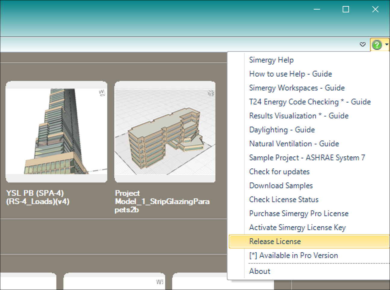
It is easy to transfer your license from one computer to another.  First you release (or deactivate) the license on the original computer.  Then you re-activate it on the new computer.  The steps are as follows:

1. Start Simergy on the original computer > click on the green “?” icon in the upper right of the application frame > select “Release License” … as shown below:
   
   

   
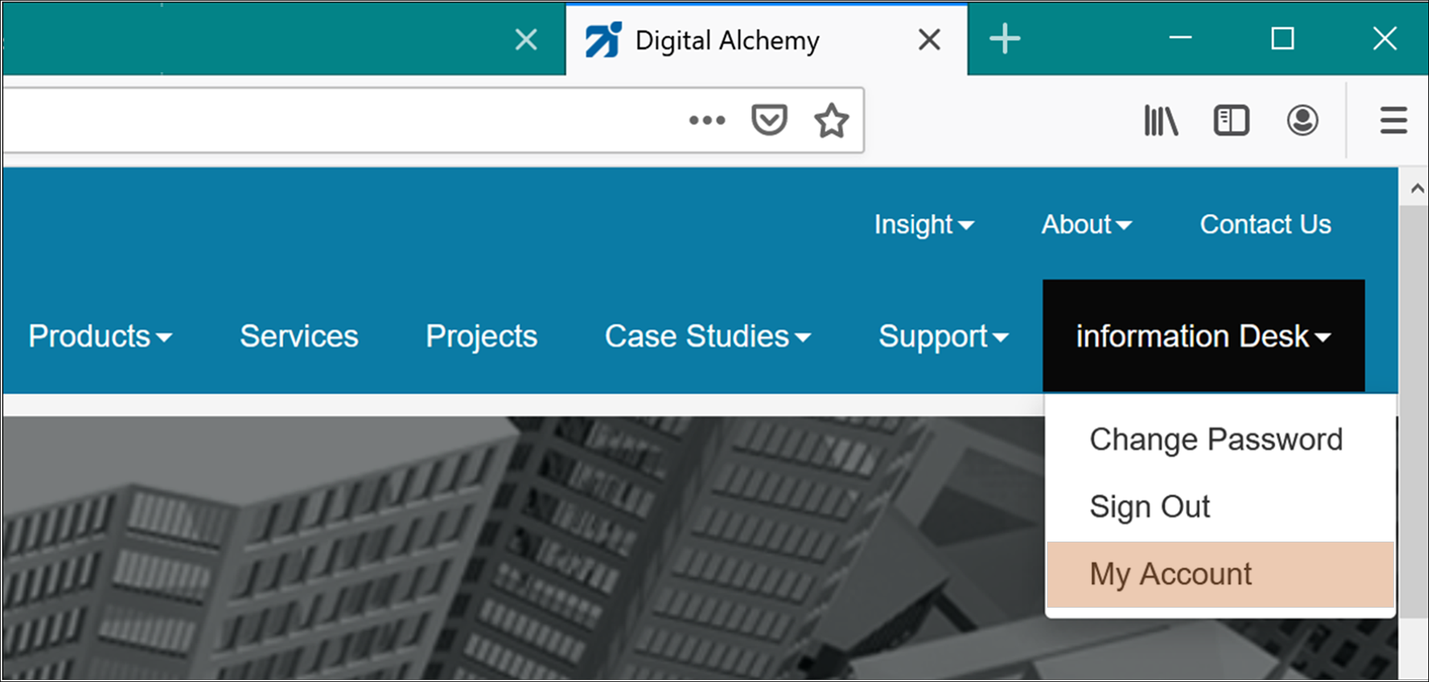
   NOTE: if you are not able to start Simergy on the original machine, please do the following:

   Browse to: https://d-alchemy.com/  > click on “Sign In” > login with the email address and password you used to register and download Simergy – after sign-in, your name will replace “Sign-In” > click on your name > select “My Account”
   
   

   This will take you to a webpage where you originally downloaded Simergy.  It contains license information for:

   • Your free Simergy Standard license
   • Your original Simergy Professional Trial license
   • Any license you purchased

   Locate the license you want to move to the new computer > click on Release License (on the right) – as shown here:
   
   

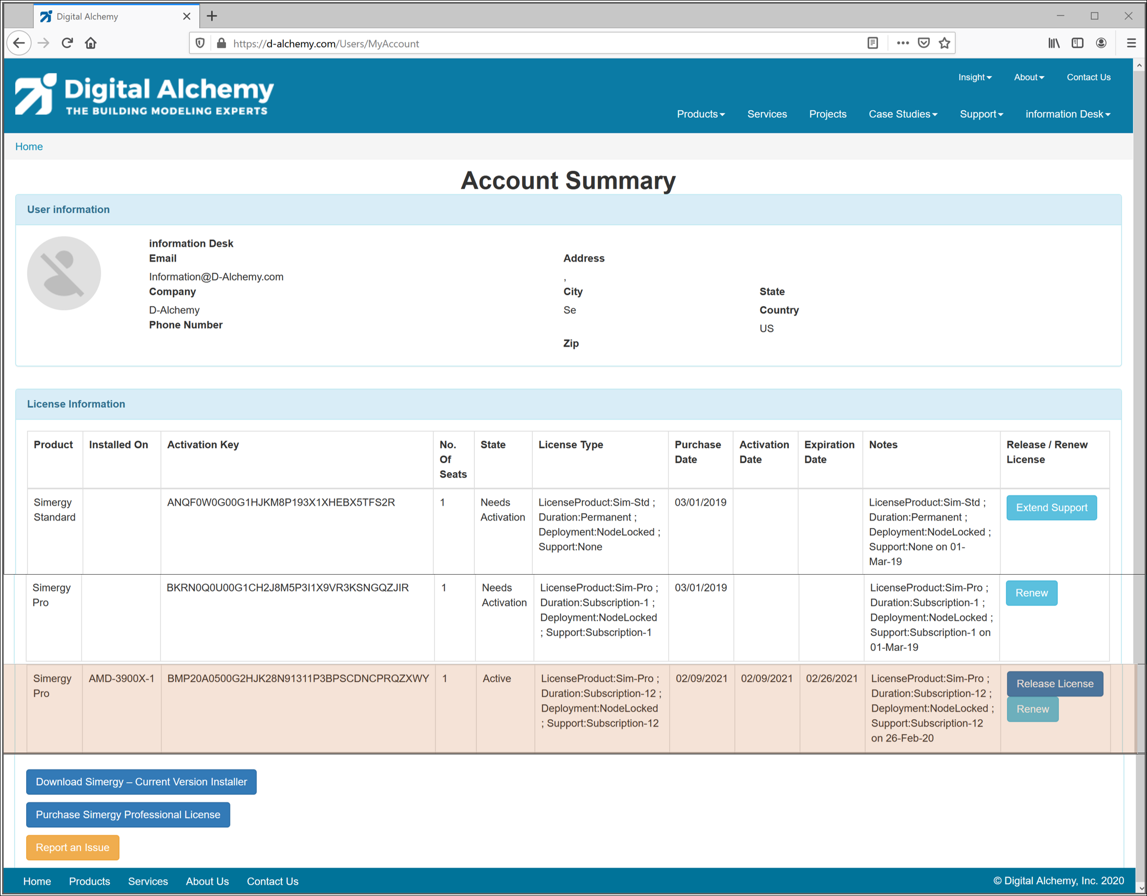
   After clicking “Release License” – it will be dis-associated from the original computer and become available to activate on the new computer.

   Copy the Activation Key from this screen.

2. Start Simergy on the new computer > click on the green “?” icon in the upper right of the application frame > select “Activate Simergy License Key” … as shown below:
   
   
   

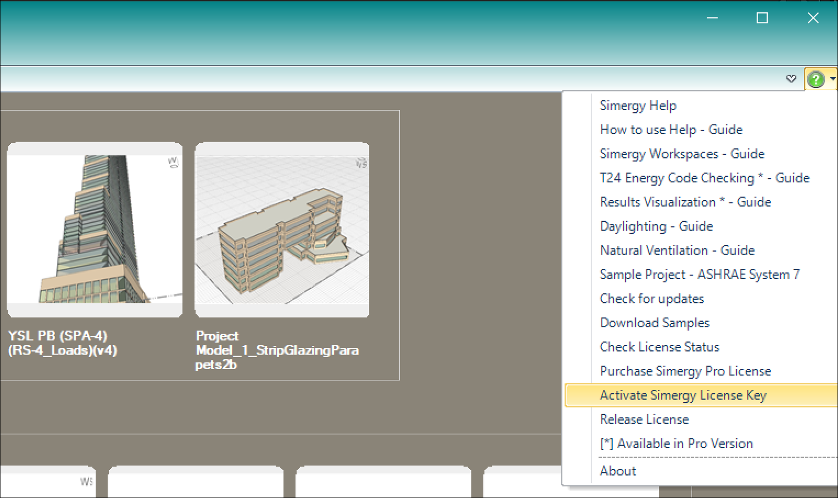
   This will launch the License Activation Wizard as shown below:
   
   

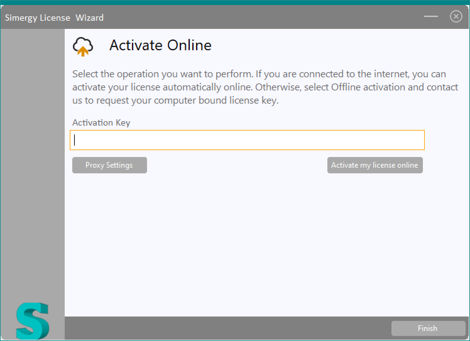
   Paste the License Activation Key that you copied from the original computer or from your “My Account” page > then click on “Activate my license online”

   Simergy will restart with the license key you pasted.  So long as the key has not expired > it will continue to work on this computer.

Yes.  To switch unit systems in Simergy projects, do the following:

1. Start Simergy > click File > New – this will load an empty project
2. Click on File > Options > User Interface Measure Units – this will display the unit system to be displayed in the UI
   
   
   
   
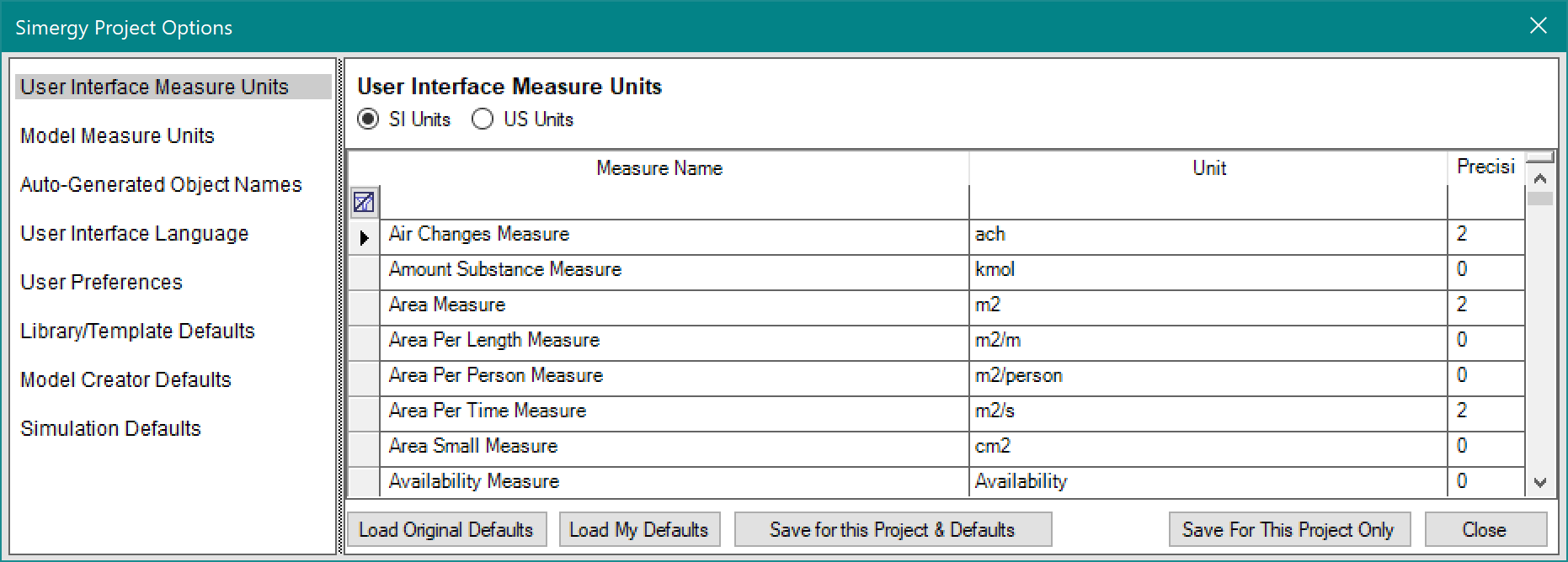
3. Click on the “SI Units” radio button at the top to use SI (metric) units or “US Units” to use US units
4. Then click on “Save for this Project and Defaults” > and then click on “Close” – both buttons are on the bottom

   This will cause all new projects to use selected unit system.

Using Custom Weather Files in Simergy

In Simergy, the weather data to be used in the energy simulation is specified on in any of the following ways:

• Project workspace

   

  

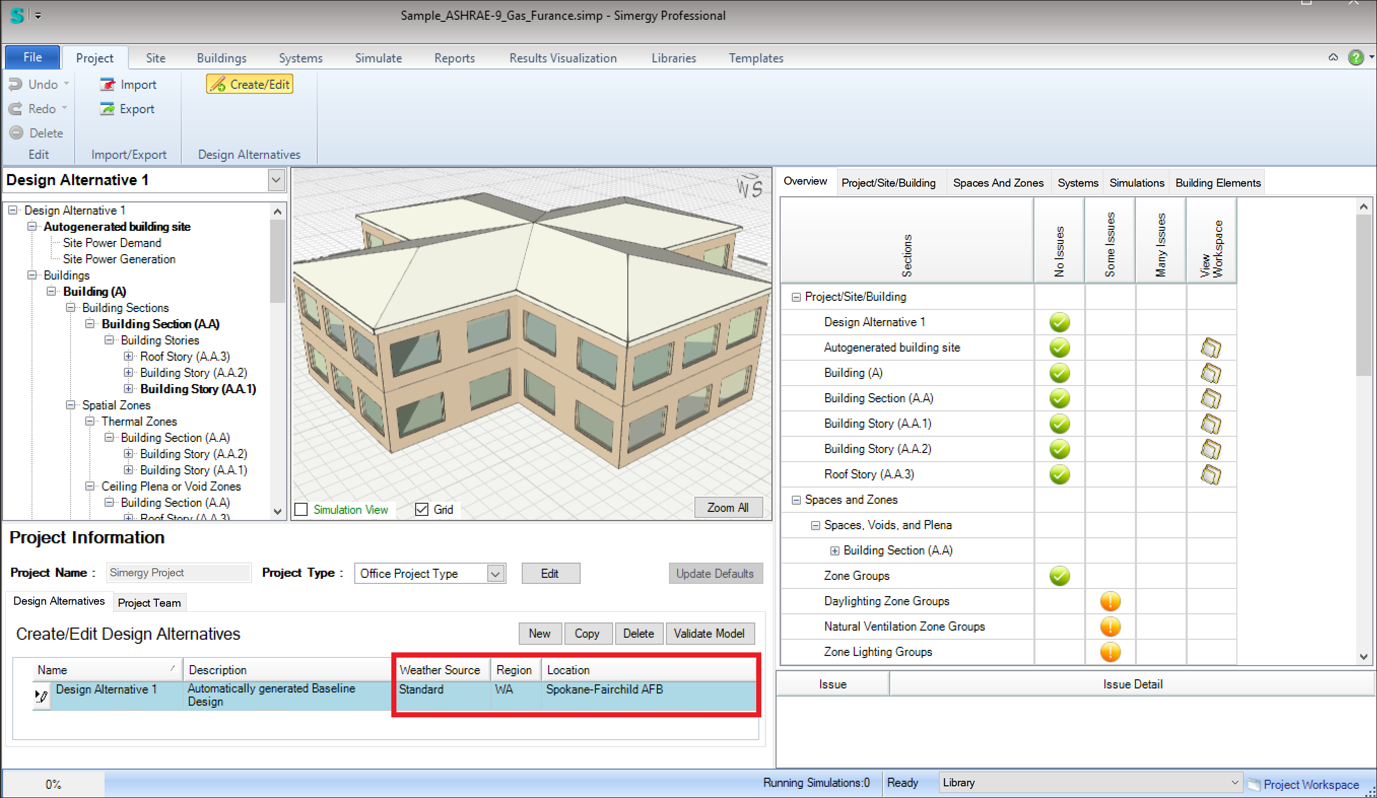
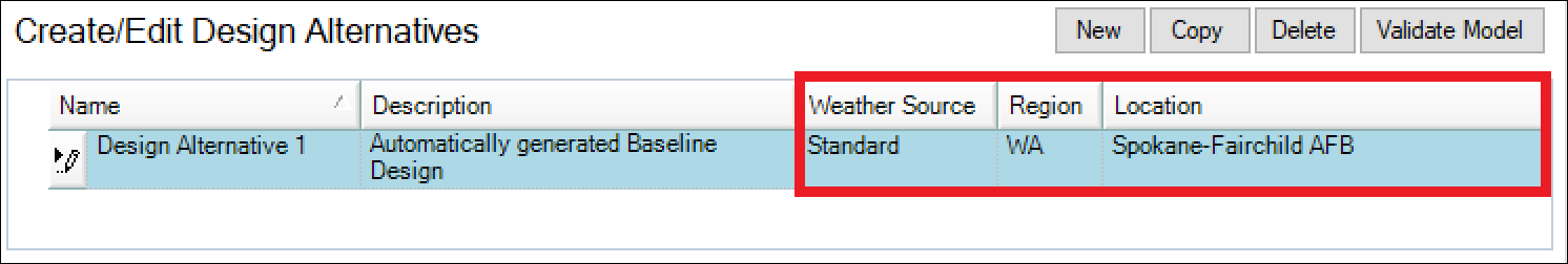
The ‘Weather Source’ field is a dropdown list allowing you to select:

• Standard (default)

  This option allows you to select one of 1,042 locations in the USA.  After selecting ‘Standard’ in the ‘Weather Source’ column > select the US state in the ‘Region’ dropdown list > then select a location in that state – in the ‘Location’ field.  The screenshot above shows the selection of WA(shington) state and then Spokan-Fairchild AFB.  Once selected, the weather data will be downloaded from a US Dept. of Energy server and copied into the Project for simulation.

• Custom

  This option allows you to select a custom weather file, typically in other parts of the world.  To use this option, first find and download the custom weather data file(s) as described below.  Then, after selecting ‘Custom’ in the ‘Weather Source’ column > browse to ‘C:\Users\Public\Simergy\WeatherFiles’ > select the .epw file.  Once selected, the weather data will be downloaded from a US Dept. of Energy server and copied into the Project for simulation.

• Simulation workspace

  

  Once you have defined a simulation configuration in the Simulate workspace, if you click on ‘Run Simulation’ and Simergy finds that you have not yet specified a location, you will be prompted to specify the location with the following dialog:

  

  As described above, for the Project workspace, you can select either ‘Standard’ or ‘Custom’ weather sources.  After making your selection, you will see more detailed information in the ‘Location metadata’ table below.

• Import workspace

  

  When you are in the Import workspace > if you import a model that does not include a location that is recognized by Simergy, you will be prompted to specify the location with the same dialog as in the Simulation workspace:

               

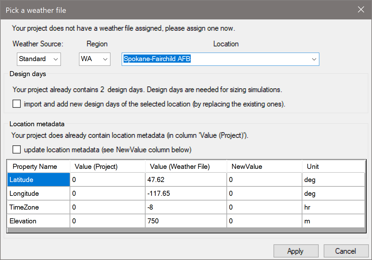
  As described above (for the Simulation workspace), you can select either ‘Standard’ or ‘Custom’ weather sources.  After making your selection, you will see more detailed information in the ‘Location metadata’ table below.

• Using Custom Weather Data

  If Simergy’s Standard weather data does not include a location for which you would like to run a simulation, you can download weather data from any of the following sources:

• EnergyPlus weather website (free): https://energyplus.net/weather

  Contains over 2,100 locations.  About half are locations in the USA and are available in Simergy’s ‘Standard’ weather source.

• Climate One Building website (free): http://climate.onebuilding.org/
• Commercial Weather website: http://weather.whiteboxtechnologies.com/

From any of these, you need to locate EnergyPlus weather files (.epw).  Once downloaded, place the file on your disk drive at: ‘C:\Users\Public\Simergy\WeatherFiles’ – which is the weather file folder used by Simergy.

Once the .epw file has been downloaded to this location, you can select it for use in your simulations using the ‘Custom’ weather source option as described above.

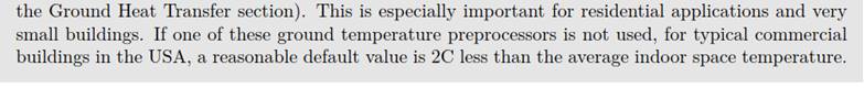
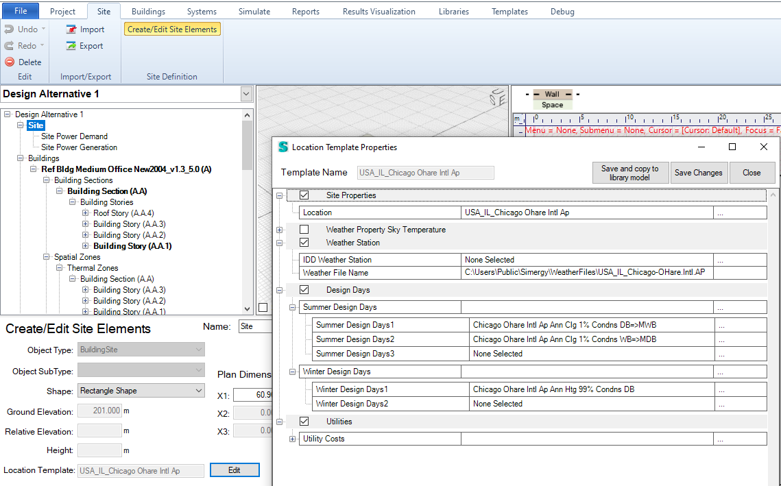
Defining ground temperatures (Site:GroundTemperature:BuildingSurface)

By default, ground temperatures are set to 18 deg C constant throughout the year. This is the simplest modelling approach.

1.      Constant default ground temperatures (one value)

2.      2 deg C above average zone air temperature (monthly)

3.      Detailed ground temperature modelling (monthly)

The EnergyPlus InputOutputReference.pdf states (p. 87):

Other ground temperatures

Other ground temperatures are mainly used for different ground heat exchangers.

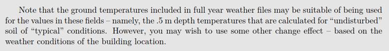
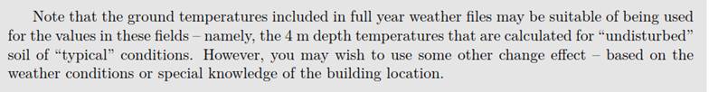
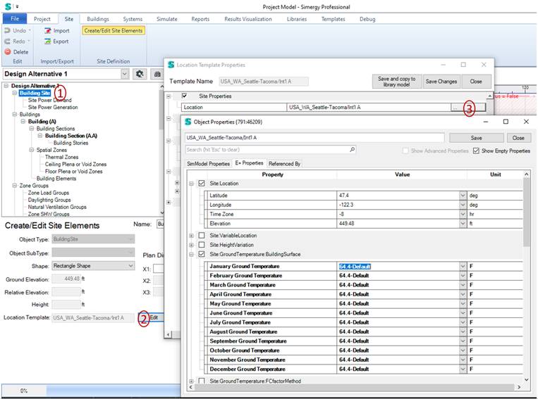
Modelling ground temperatures (Site:GroundTemperature:BuildingSurface)

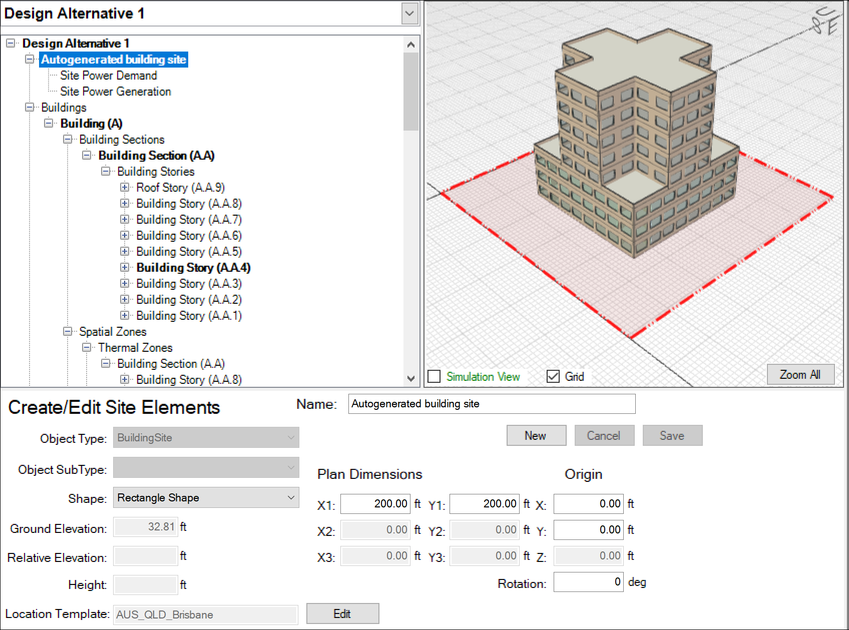
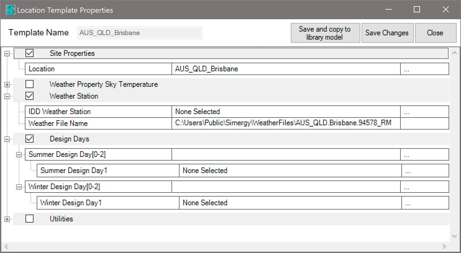
The first two can be easily defined in Simergy (first one is the default), second option can be defined in the location template (either taking temperature setpoints into account or adding report variables to actually report monthly temperatures in the zones):

Site Workspace

1.     Select the Building Site in the tree

2.     Click on the Edit button next to Location Template

3.     Click on the … Button

The detailed ground modelling is not directly supported in Simergy 4.0 yet but is on the enhancement list.

 In the project workspace

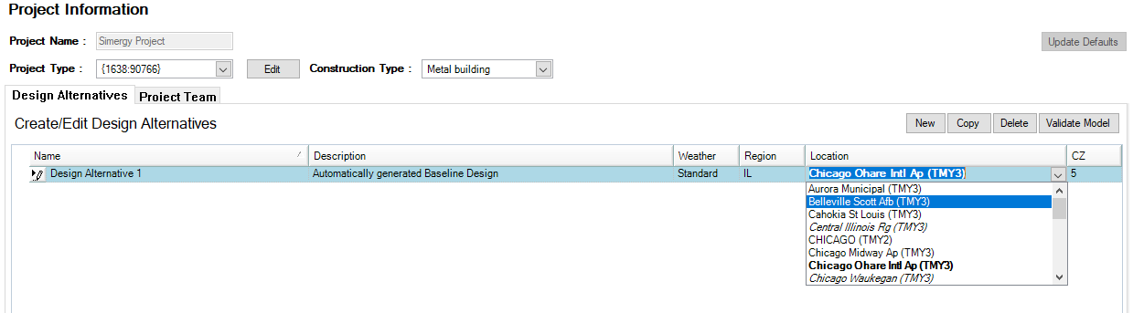
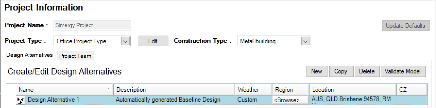
When you use the Standard Weather Source and select a US region the location dropdown contains a list of all locations of that region, which are formatted in the following way:

• [normal] rows are normal
• [italic] rows indicate that this location does not have design days
• [bold] indicates that this weather file was already downloaded and it available on the current PC (in C:\Users\Public\Simergy\WeatherFiles)
• [UPPER CASE] rows indicate the older TMY2 format
• (TMY-2-3) In brackets we show the TMY version, TMY, TMY2 and TMY3 (TMY3 being the newest weather file version)

The CZ column contains the ASHRAE climate zone that is automatically determined based on the weather location if possible.

This document will explain how to define utility cost in a Simergy model: by illustrating the assigned of a utility cost object to a project, by creation of a utility cost object in the library and via an example.

1. Assigning utility cost objects to a project

• Go to the Site workspace
• Click on Site in the project tree
• Click on the Edit button right next to “Select Location”
• In the Locations template check the checkbox for Utilities.
• Select all utility tariffs you want to assign to this project.

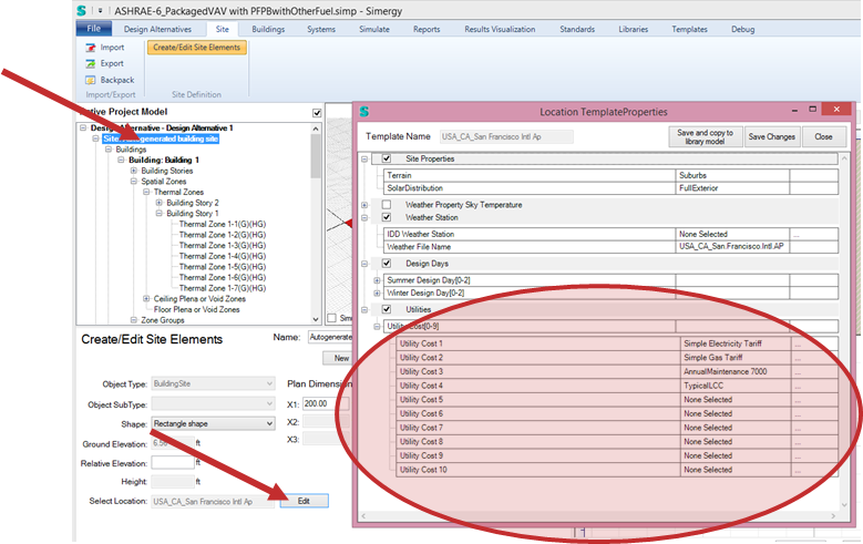
                                                   Figure 1: Steps to assign a utility tariff to a Simergy project

2. Create utility tariff object(s) in the library

For each energy source (e.g. Electricity, Gas, …), you need to define a Utility Tarif object (Type: UtilityCost Subtype: Tariff) in the library workspace under Location Data and Costs. Each of those Utility Tariff objects is assigned to a Meter that links the cost to the related energy consumption of that meter. You can use any meter from the meter dropdown, but usually one would use a meter at the facility level. Each Utility Tarif object then is referenced by a number of other cost objects that define the cost structure of the tariff. For example, with a cost variable object one can assign a monthly cost value and with a Charge Simple object a simple cost per unit (e.g., 0.5 $ per kWh). Figure 2 illustrates the relationships between these cost objects.

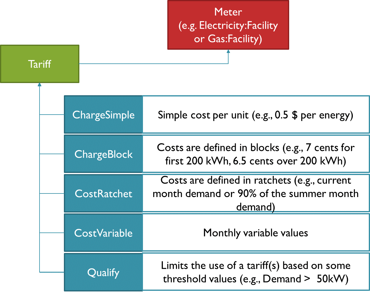
                                                                    Figure 2: Utility cost objects

3. Example tariff

In the below table is an example tariff defined that has a constant monthly charge as well as a constant demand charge. Furthermore, this tariff is different for summer and winter for the energy consumption and uses on, mid and off peak rates.

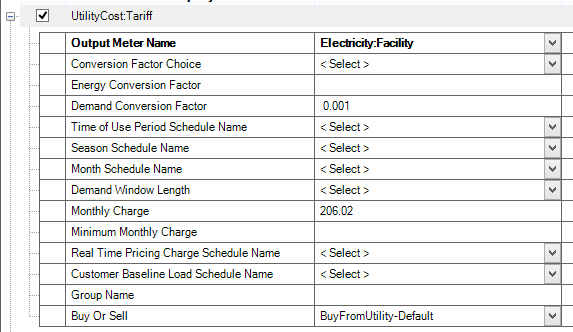
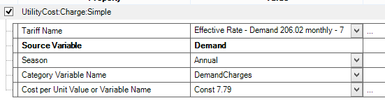
For the demand side, we define a Tariff (Type: UtilityCost Subtype: Tariff) object (called Effective Rate – Demand 206.02 monthly – 7.79 per kW) that contains the monthly charge of 206.02.

This demand tariff object is defined by the SimpleCharge object (Type: UtilityCost Subtype: ChargeSimple), which specifies the Category Variable Name as demand charge, provides a constant cost value and sets the season to annual to make this demand applicable for the full year.

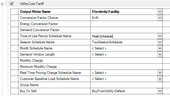
For the consumption part we define another tariff object (Type: UtilityCost Subtype: Tariff), see below:

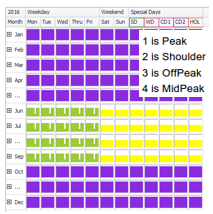
This tariff object references two schedules, a schedule that defined the different peak categories and a schedule that differentiates between summer and winter. See the related peak schedule to the right.

In addition, three Simple Charge objects (Type: UtilityCost Subtype: ChargeSimple), are linked to the Electricity Rate – Consumption tariff object. They define the cost value, are bound to the season (here summer) and to the peak category.

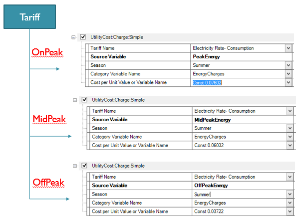
Finally, one SimpleCharge object (Type: UtilityCost Subtype: ChargeSimple), for the winter season would complete this example.

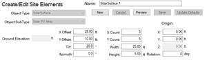
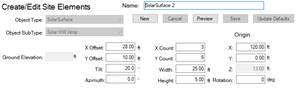
Solar surfaces

For PV and solar thermal components, we first need solar surfaces. These are created in the Site workspace. For PV units you need to create a SolarSurface with subtype “Solar PV Array” and for solar thermal components you need to create a SolarSurface with subtype “Solar HW Array”. Note that for each surface, we will create a separate PV unit or thermal collector.

Moving solar surfaces (on the roof)

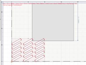
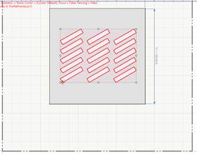
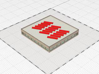
Once you have placed your solar surfaces, you can also move them onto the roof or around your site.

Click the anchor on the lower left of the shape. Release the left mouse button, now you can drag the surface array around. To get it onto the roof just click on it and it will automatically be placed on top of it. Below you can see them properly placed in 3D.

PV and solar collector reference solar surfaces

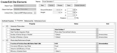
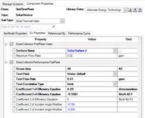
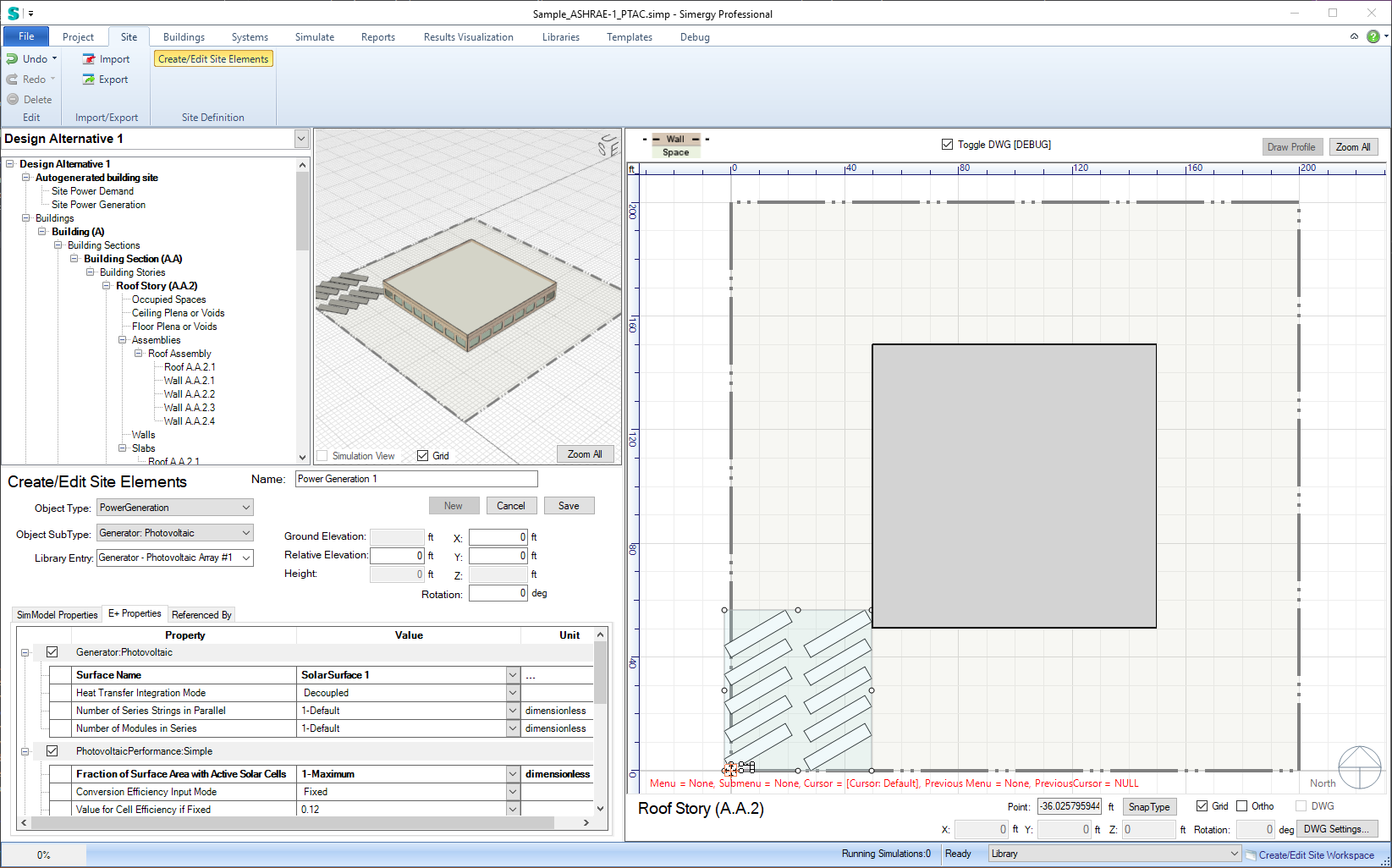
Both the PV and solar thermal component then reference those surfaces in the Surface Name property:

Creating a PV:

The PV is also generated in the Site workspace, under PowerGeneration and Generator:Photovoltaic. Besides the already discussed Surface Name property. You can choose from one out of three PhotovoltaicPerformance options: Simple, EquivalentOne-Diode and Sandia. Note it is important that you only check one of these.

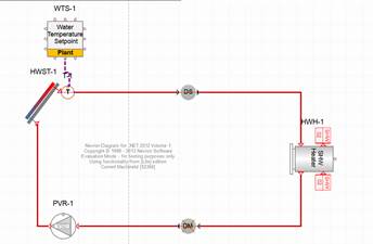
Creating Solar Thermal:

Typically, solar thermal components are used in context of service hot water and in combination with a water tank. To model this in Simergy, we typically create two loops one with a water tank that connected to the service hot water demand and another one that connects that water tank with the solar collector. This way the solar collector can store the generated heat in the tank and the tank can provide hot water when needed as service hot water. The tank also has another heat source in case the solar collector cannot provide enough. The solar collectors can also be part of hot or mixed water loops or more complex water systems with cross connected heat exchangers between system types.

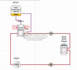
Simergy supports three different collector types:

1.       SolarCollector:FlatPlate:Water

2.       SolarCollector:IntegralCollectorStorage

3.       SolarCollector:FlatePlate:PhotovoltaicThermal

The first one is the standard collector, the second one already integrates a small storage tank and the last one is a combined hot water collector and PV unit.

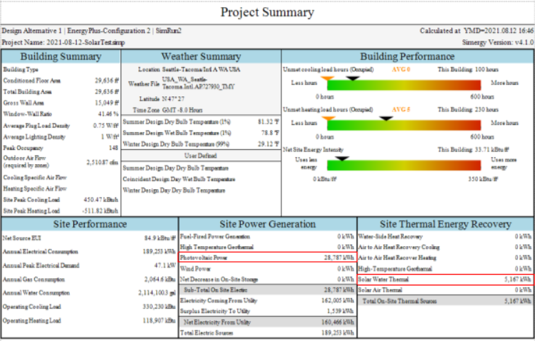
Results and Reports

The project summary report contains data about the performance of PV units and solar collectors. Site Power Generation section shows the Photovoltaic Power generated and the Site Thermal Energy Recovery section the Solar Water Thermal energy. These values provide a quick overview of the performance, but of course more details are available in other reports and variables in results visualization.

Photovoltaics in Simergy

First, we need to create a surface array in the Site workspace:

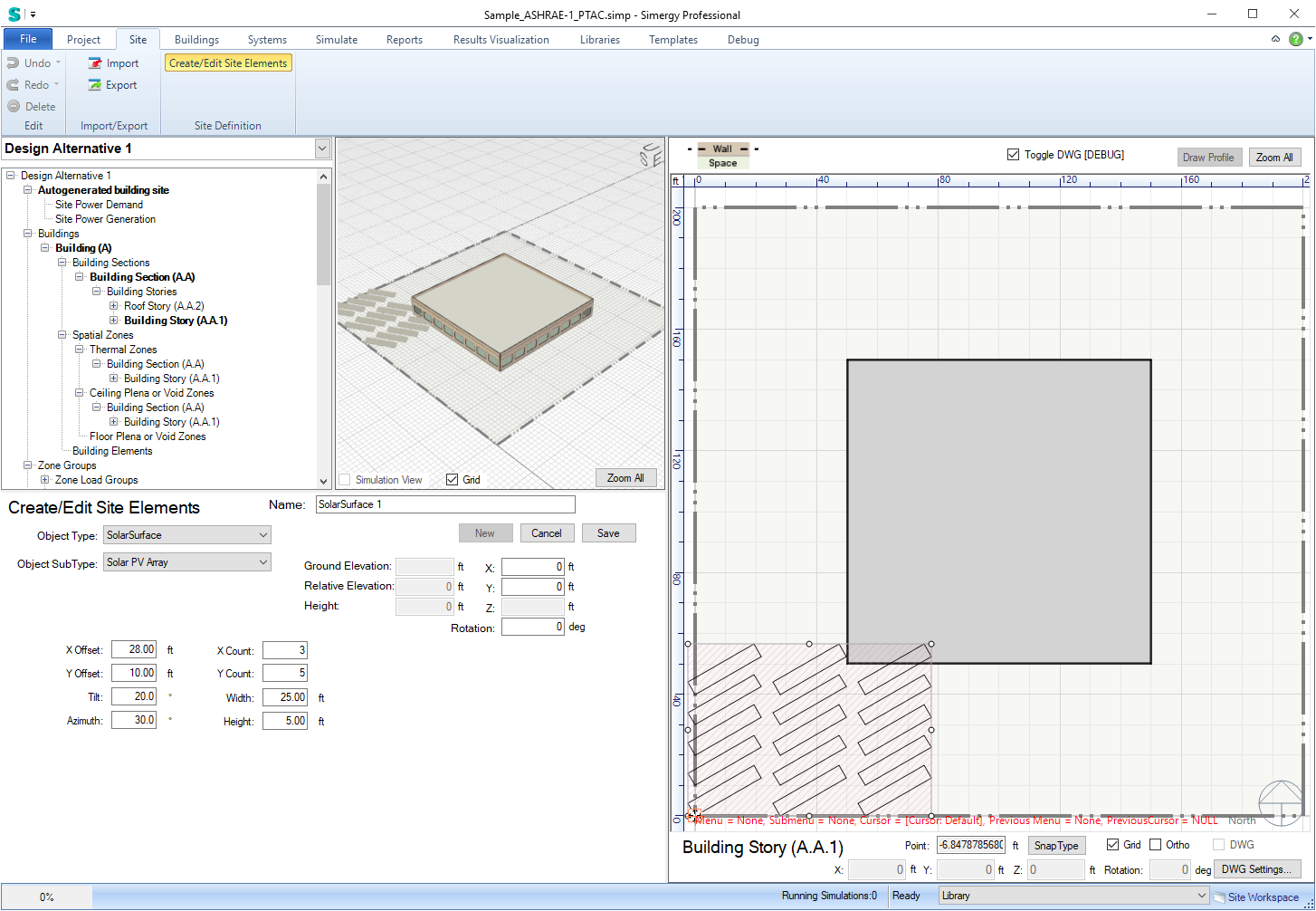
Then we create a Generator:Photovoltaic and select the just created solar surface in Surface Name.

Example for creating below grade building stories:

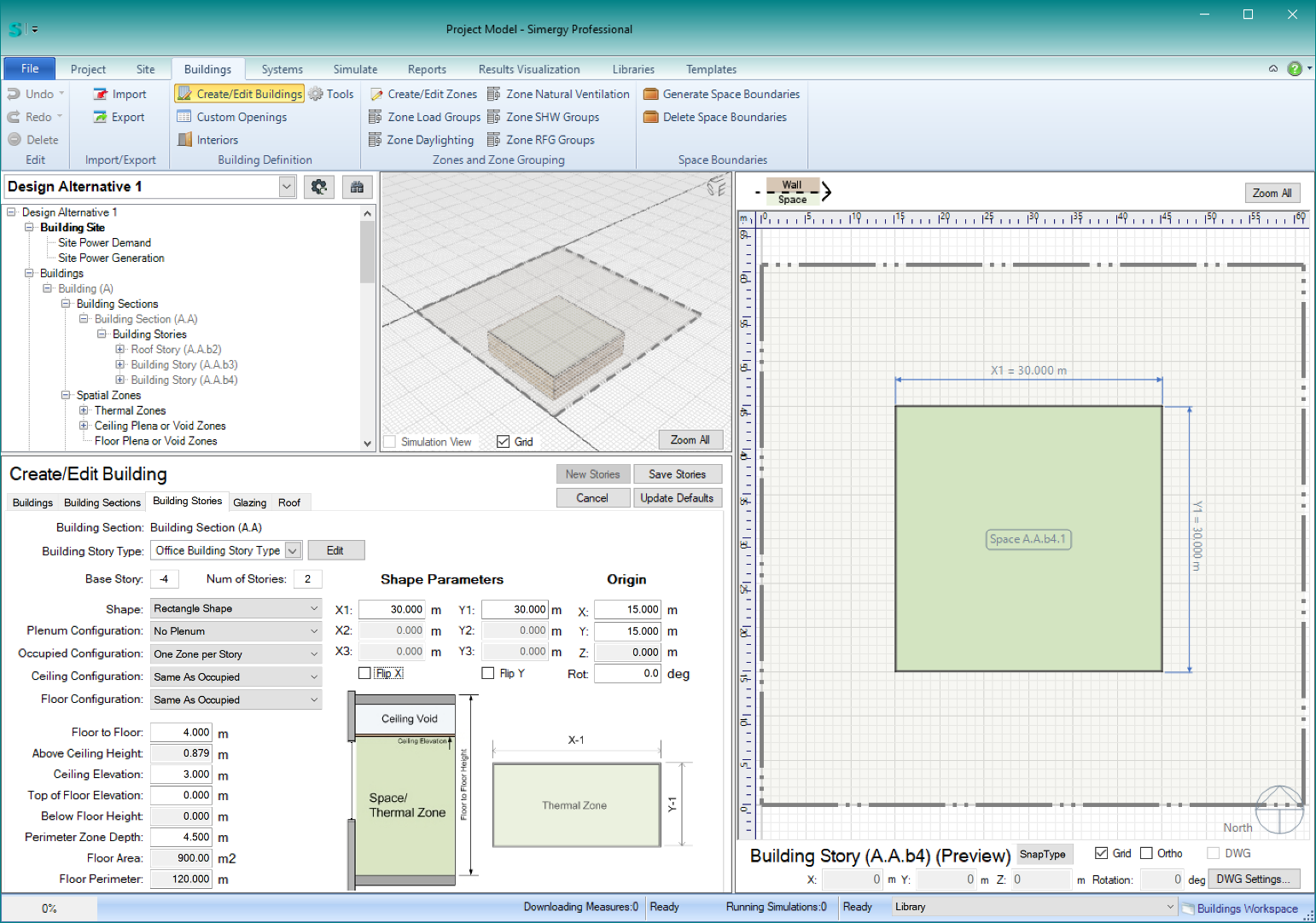
1. Let’s say you want a total of (4) rectangular basement stories – using 4m floor-to-floor height and 3m ceiling elevations, but you want the bottom (2) basements to be 30m x 30m, and the top (2) basements to be 35m x 35m (center aligned), with (1) zone per story … and then you wanted 10 stories above grade with similar parameters.
2. Currently, you need to start with the lowest story, so you parameters for basements 3 & 4 would look like this: (note the the ‘Base Story’ index is -4)
   
   
   

   To complete these basement stories, simply click ‘Save Stories.’

3. After saving those stories , you parameters for basements 1 & 2 parameters would look like this: (note the the ‘Base Story’ index is -2)
   
   
   

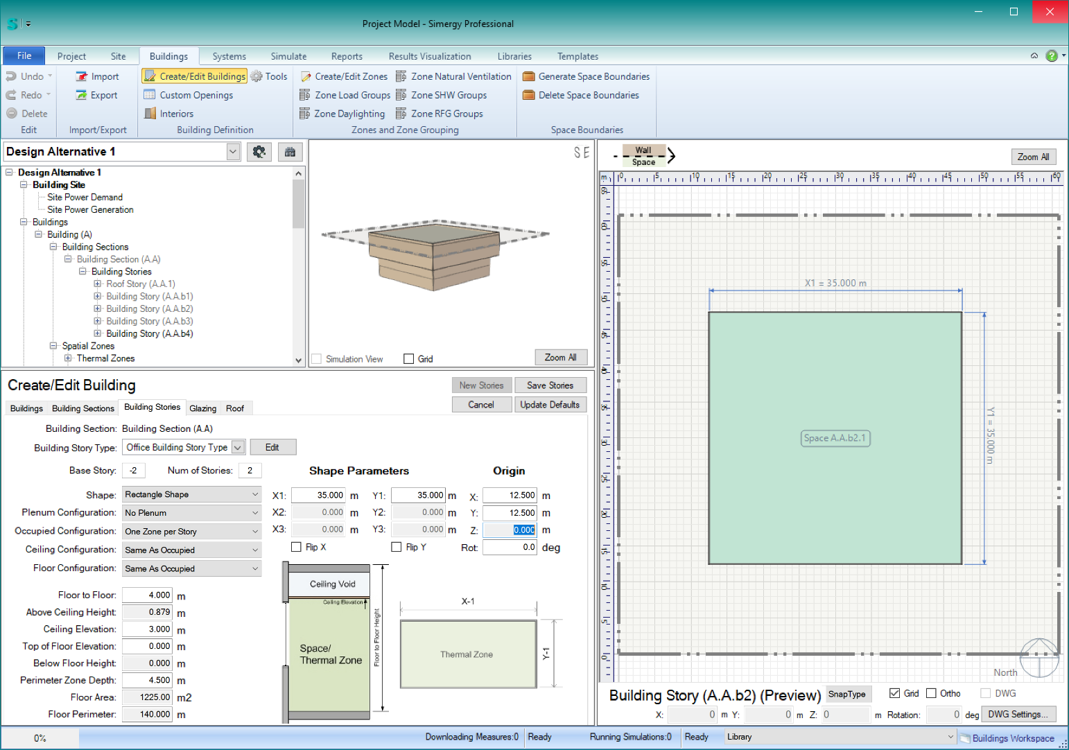
   To complete these basement stories, simply click ‘Save Stories.’

4. Then – to add the (10) stories above grade, you parameters might look like this:
   
   
   

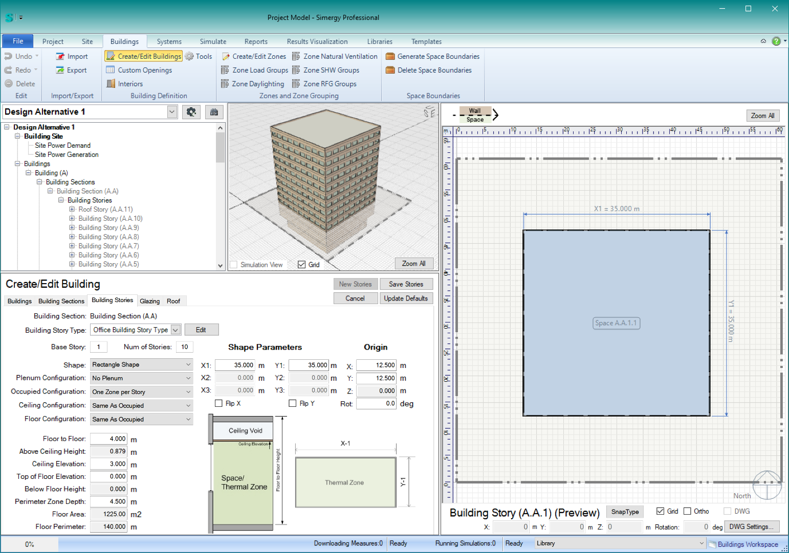
   To complete the building, simply click ‘Save Stories.’

Courtyards in Buildings (as shown in the screenshot below)

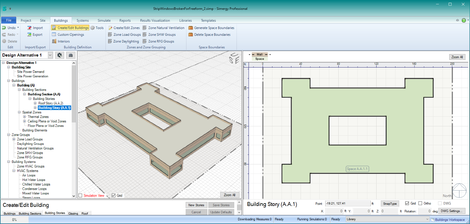
Steps for Creating a Courtyard:

1. File > New > Buildings > New Stories
2. Set number of stories > Set all the other parameters except shape > then set shape to Freeform – this will put you into ‘draw mode’ in the plan view
3. Take note of the controls above the plan view when in ‘draw mode’ (see screenshot below).
   
   

   

    

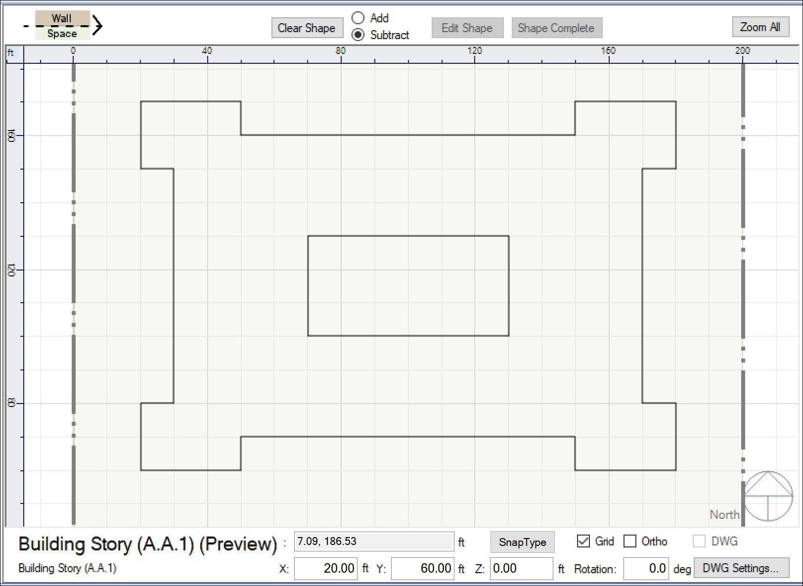
   These controls allow you to perform Boolean operations on the shapes you draw – using the “Add” and “Subtract” radio buttons.  First select “Add” mode and draw the outer walls of your building > then select “Subtract” mode and draw the courtyard shape.  As you are drawing a loop, if you mis-click > click Control+Z to undo the last point clicked.  If you want to edit the shapes more, use the “Add” and “Subtract” to modify the shapes.  When you are happy with the shapes > click on “Shape Complete.”  This will tell the Building Model Creator™ to create the building stories.

   NOTE-1: You can create multiple courtyards, by creating multiple inner-loops using “Subtract.”

   NOTE-2: If you want to modify these shapes at a later time (i.e. a design change), do the following:

   1. Select the building story in the tree – this will load all the parameters for this building story
   2. Change any parameters other than shape first (e.g. floor to floor height, ceiling height, glazing parameters
   3. To then change the freeform shapes > click on “Edit Shape” above the plan > make changes using the Boolean operations as you did when you created the original shapes.

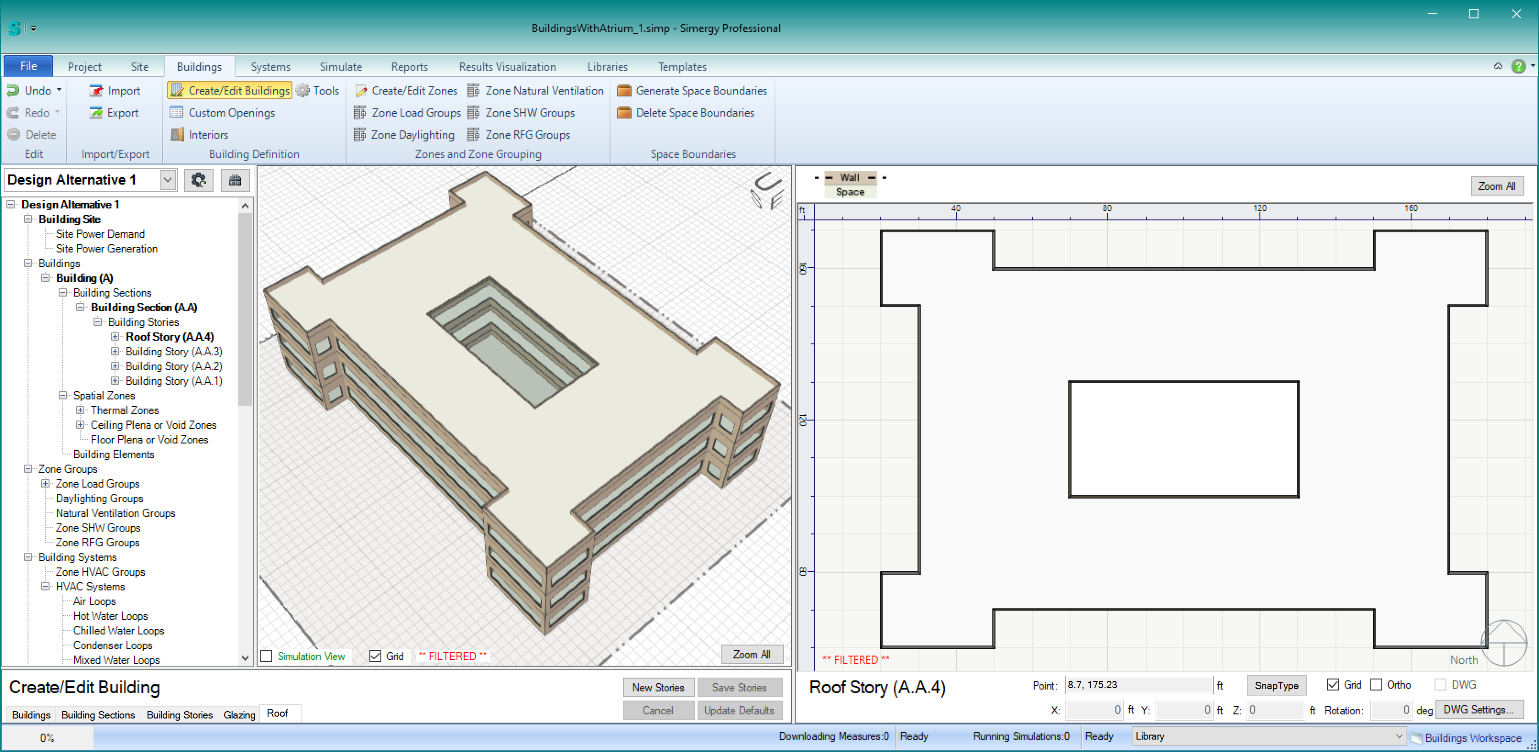
Atriums in Buildings (as shown in the screenshot below)

Steps for Creating a Courtyard:

1. File > New > Buildings > New Stories
2. Set number of stories > Set all the other parameters except shape > then set shape to whatever you want (this example uses ‘Freeform’) > click “Save Stories to save the building stories.
3. Select the building story 2 (if Building is A and Section is A, this would be named A.A.2)
4. Click on the Tools workspace under Buildings: 
   
   

   

   

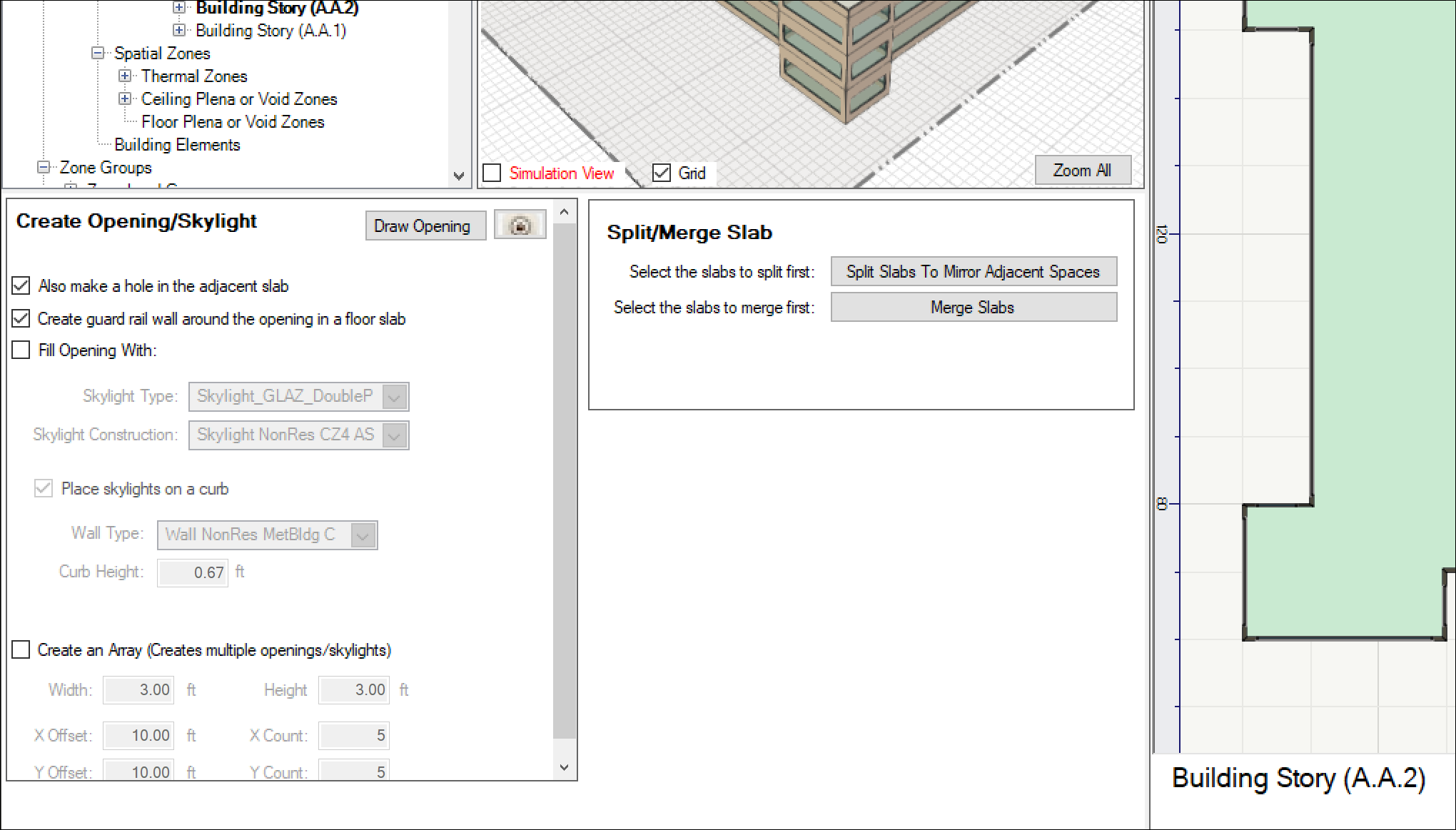
   The Tools palette is in the lower left.  You can use these tools to make holes in floor, ceiling, and roof slabs.  There are also settings that enable generation of additional objects, including: skylights, curbs under the skylights, shaft walls around openings going through ceiling spaces, guardrails around openings in floor slabs.  You can also create arrays of openings or skylights.

5. Select the checkboxes you want in the ‘Create Opening/Skylight panel > then click on “Draw Opening” button < this will put you into drawmode in the Plan view. Draw your opening snapping to the grid or freeform.  When the loop is closed, the opening(s) will be made.  If you selected the “Also make a hole in adjacent slab,” All of the following will be done:
   • Openings in both the floor slab and the ceiling slab below
   • Shaft walls will be made connecting those two openings and surrounding the shaft
   • The shaft will be filled with a new space called “

   If you selected “Create guard rail walls around opening in floor slab” – such walls will be created around the opening

   Note: it is possible to ‘Fill Opening with” a skylight assembly, but this is normally only done for roof slabs

   When done, you now have an atrium connecting the first and second building stories and should see something like this:
   (note: we have hidden stories and roofs above story 2 in this screenshot)

   
   

   

   
   
   
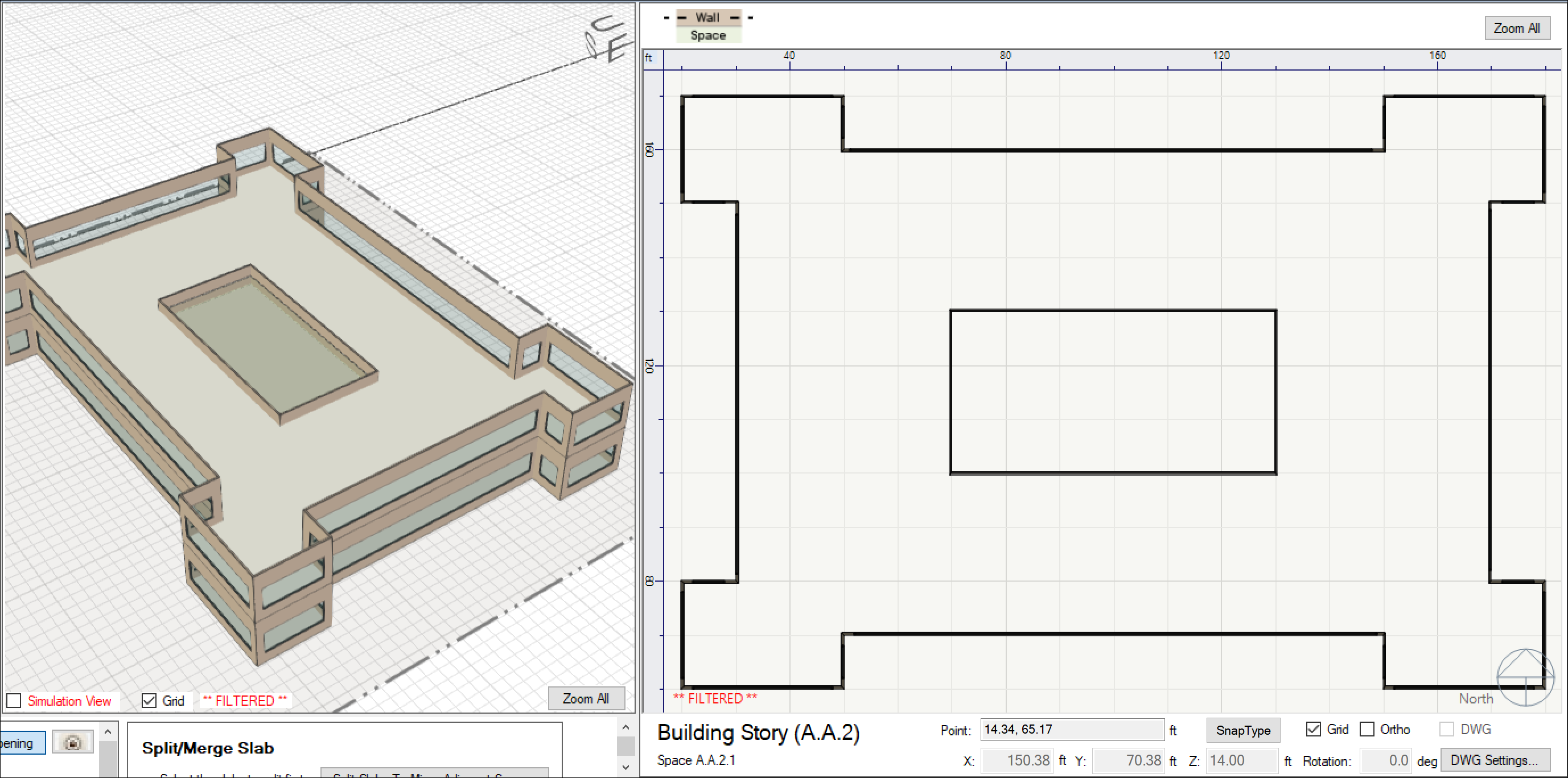
6. Repeat step (5) for as many stories as you wan the Atrium to connect. NOTE: when drawing the openings on stories above, you can snap to the corners of the openings you have already created below.
7. To add a skylight in the roof above this atrium > select the Roof Story > select the “Fill Opening With” checkbox > select the Skylight Type’ you want, and repeat the “Draw Opening” process you did for the stories below. The end result should look something  like this:
   
   

   

Simple and detailed natural ventilation

There is a simple and a detailed natural ventilation option in Simergy. The simple approach is defined at the zone level and very flexible the detailed approach is using a network of nodes that all must be connected.

Simple natural ventilation

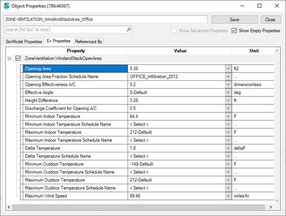
The simple natural ventilation is implemented in Simergy on a zone level with the EnergyPlus object: “ZoneVentilation:WindandStackOpenArea” (see documentation here: https://bigladdersoftware.com/epx/docs/9-2/input-output-reference/group-airflow.html#zoneventilationwindandstackopenarea). This simplified approach determines the ventilation air flow rate as a function of wind speed and thermal stack effect. This simple approach does not require anything else than this object to one or more thermal zones in the model. There is no interconnectivity.

Defining natural ventilation templates

Both natural ventilation templates can be either defined at the building level (Building workspace -> Building tab) or via Zone Natural Ventilation groups. While for the simple natural ventilation only a library object is referenced for the detailed natural ventilation a template object is referenced.

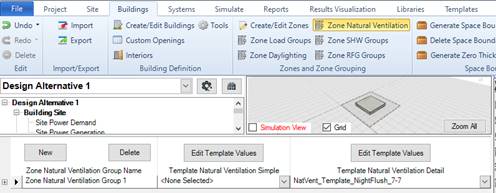
Detailed natural ventilation

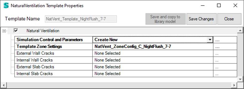
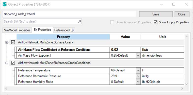
The detailed natural ventilation requires the specification of a NaturalVentilation Template object that defined NatVEnt controls, Zone Settings as well as possible cracks. In addition to this template opening properties can also be attached to windows and doors.

You need to define this node based detailed natural ventilation in a way that all nodes are connected. That means each zone that is assigned to a natural ventilation template must have at least two nodes (either opening or crack) and the resulting nodes must be connected.

Detailed about all related object and parameters can be found here: https://bigladdersoftware.com/epx/docs/9-2/input-output-reference/group-airflow-network.html#group-airflow-network

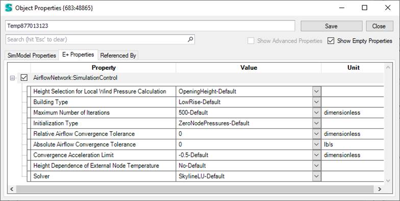
The basic run parameters for this model are defined in this unique simulation control object. Currently, in Simergy only the SurfraceAverageCalculation option for the wind pressure coefficients is supported.  

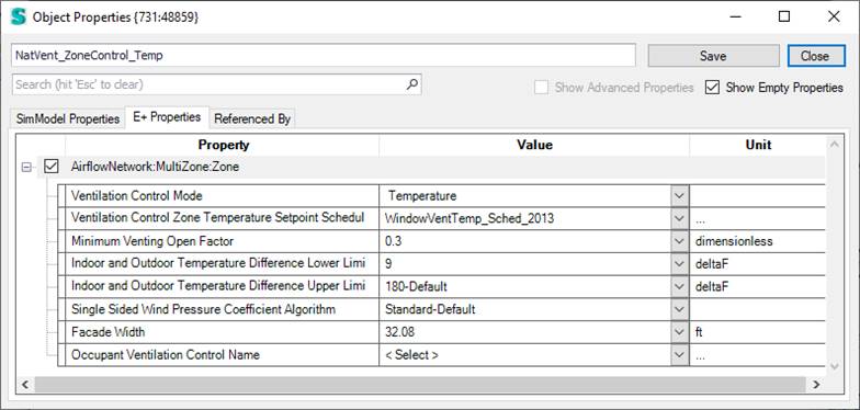
The AirflowNetwork:MultiZone:Zone object allows control of natural ventilation through exterior and interior openings in a zone, where “opening” is defined as an openable window or door.

This object is required to perform Airflow Network calculations. Note that ventilation control for all openings is provided at the zone level.

Different Opening types

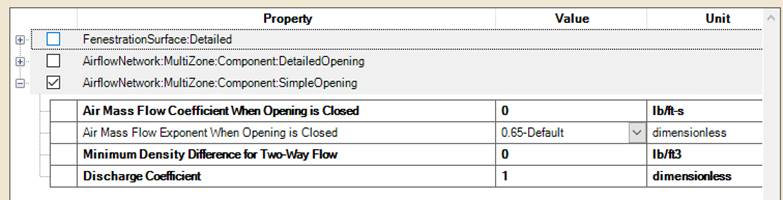
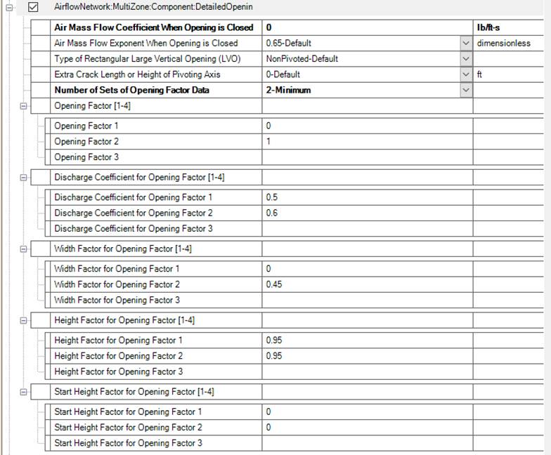
There are 3 different opening types:

1.      SimpleOpening

2.      DetailedOpening

3.      HorizontalOpening

Those opening properties are attached to windows or doors. You can use existing library entries by using Window or DoorTypes. Simergy is automatically generating AirFlowNetwork:Surface objects that related to these openings. Other air flow network objects in EnergyPlus are currently not supported in Simergy.

The SimpleOpening object specifies the properties of air flow through windows, doors and glass doors (heat transfer subsurfaces) when they are closed or open. The AirflowNetwork model assumes that open windows or doors are vertical or close to vertical.

The DetailedOpening object specifies the properties of air flow through windows and doors (window, door and glass door heat transfer subsurfaces) when they are closed or open. The fields are similar to those for SimpleOpening object when the window or door is closed, but additional fields are required to describe the air flow characteristics when the window or door is open. These additional fields include opening type, opening dimensions, degree of opening, and opening schedule.

This object specifies the properties of air flow through windows, doors and glass doors (heat transfer subsurfaces defined as a subset of FenestrationSurface:Detailed objects) when they are closed or open. This AirflowNetwork model assumes that these openings are horizontal or close to horizontal and are interzone surfaces. The second and third input fields are similar to those for SimpleOpening/DetailedOpening when the window or door is closed, but additional information is required to describe the air flow characteristics when the window or door is open. This additional information is specified in the last two input fields. The airflow across the opening consists of two types of flows: forced and buoyancy. The forced flow is caused by the pressure difference between two zones, while the buoyancy flow only occurs when the air density in the upper zone is greater than the air density in the lower zone. This opening also allows for the possibility of two-way flow when forced and buoyancy flows co-exist.

By default, the Room Air Model in EnergyPlus and Simergy is well mixed. This assumes the temperature (and other parameters) are constant within each zone. However, there are several options to vary room air:

1. OneNodeDisplacementVentilation
2. ThreeNodeDisplacementVentilation
3. CrossVentilation
4. UnderFloorAirDistributionInterior
5. UnderFloorAirDistributionExterior

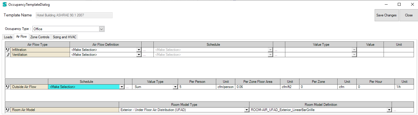
All those models can be defined within the Occupancy Template, specifically on the “Air Flow” tab. The user can select one of the five detailed room air models and then select a related library entry that is applied to each zone that is part of the zone group of this template.

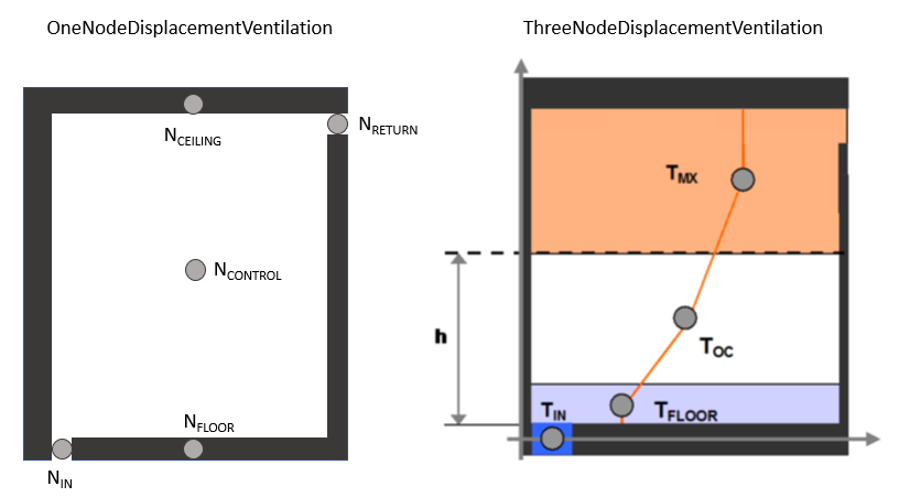
OneNodeDisplacementVentilation

The Mundt one node displacement ventilation air model for displacement ventilation defines two fractions and five nodes that are automatically generated by Simergy (see left figure below).

ThreeNodeDisplacementVentilation

“This model is applicable to spaces that are served by a low velocity floor-level displacement ventilation air distribution system. Furthermore, the dominant sources of heat gain should be from people and other localized sources located in the occupied part of the room. The model should be used with caution in zones which have large heat gains or losses through exterior walls or windows or which have considerable direct solar gain. The model predicts three temperatures in the room (see right figure below):

• A foot level temperature (TFLOOR). The floor region is 0.2 meters deep and TFLOOR represents the temperature at the mid-point of the region.
• An occupied subzone temperature (TOC), representing the temperature in the region between the floor layer and the upper, mixed layer.
• An upper node representing the mixed-layer/outflow temperature (TMX) essential for overall energy budget calculations and for modeling comfort effects of the upper layer temperature.” (From the InputOutputReference.pdf)

CrossVentilation

“The UCSD Cross Ventilation Room Air Model provides a simple model for heat transfer and temperature prediction in cross ventilated rooms. Cross Ventilation (CV) is common in many naturally ventilated buildings, with air flowing through windows, open doorways and large internal apertures across rooms and corridors in the building.” (From the InputOutputReference.pdf)

This option will only work in combination with natural ventilation. Please ensure that the zones you define cross ventilation for are also part of the natural ventilation network.

UnderFloorAirDistributionInterior

“This model is applicable to interior spaces that are served by an underfloor air distribution system. The dominant sources of heat gain should be from people, equipment, and other localized sources located in the occupied part of the room. The model should be used with caution in zones which have large heat gains or losses through exterior walls or windows or which have considerable direct solar gain. The model predicts two temperatures in the room:

• An occupied subzone temperature (TOC), representing the temperature in the region between the floor and the boundary of the upper subzone.
• An upper subzone temperature (TMX) essential for overall energy budget calculations and for modeling comfort effects of the upper layer temperature.” (From the InputOutputReference.pdf)

UnderFloorAirDistributionExterior

“This model is applicable to exterior spaces that are served by an underfloor air distribution system. The dominant sources of heat gain should be from people, equipment, and other localized sources located in the occupied part of the room, as well as convective gain coming from a warm window. The model predicts two temperatures in the room:

• An occupied subzone temperature (TOC), representing the temperature in the region between the floor and the boundary of the upper subzone.
• An upper subzone temperature (TMX) essential for overall energy budget calculations and for modeling comfort effects of the upper layer temperature.” (From the InputOutputReference.pdf)

Applying dynamic shading control to windows

1.     Single windows

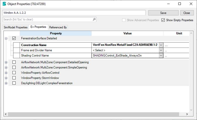
To get to the shading properties, select one or more windows and right click Properties.

In this property dialog there is one Property called “Shading Control Name” that hold the reference to a so-called shading controller in this case: “SHADINGControl_ExtShade_AlwaysOn”.

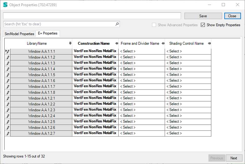
2.     Multiselect

You can also multiselect windows and use the same property dialog from above to assign shading controls. Either by selecting the manually or by using the select options in the right click menu.

3.     Edit windows in table

The third option is to use the Edit in Table right click menu option to get an overview of all the windows and their properties. Here it is also easy to apply a shading control to just the windows needed.

4.     Window Type

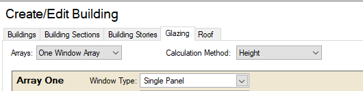
You can also attach the shading controller to a window type that you can use in the Building Model Creator^TM so that the shading can be applied to all windows right from the moment you generate the building model or later when you edit it.  You can find this option in the Glazing tab.

Shading location

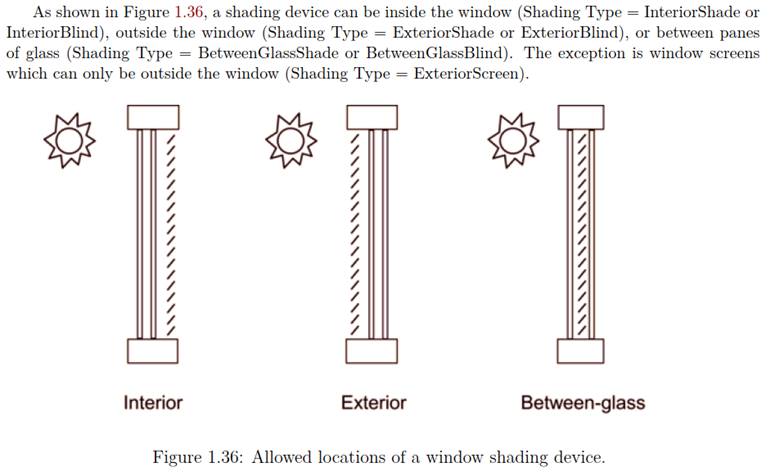
Shading types

The following tables summarizes the available shading types. Specifies the location, the related material/construction, and other requirements. There are two ways depending on your shading type either you need to define just the shading material layer that gets added to the existing window construction or you need to define a new construction with the shading device included. In the later case, the construction on the window and the construction on the shade controller need to be different just in the shading layer. For in between shading, you can obviously just use it with a double or triple glazing construction.

Shading control types

The following tables describes the details on different shading control types.

In the systems workspace

We use several acronyms in our HVAC templates, see below for descriptions:

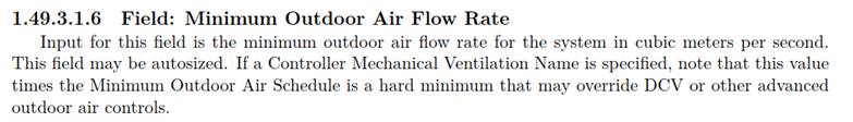
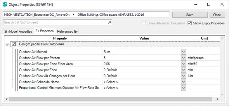
Defining outdoor air flow

In Simergy/EnergyPlus there are various ways to define outdoor air requirements. The so-called Design Outdoor Air Specification object allows to define the air flow per floor area, per person, per zone, and per hour (etc.).

This object can be referenced by various components as shown in the figure below. At the system level in the Idea load object or in an air loop at the outside air controller. At the zone level at some of the air terminals and for zone sizing.

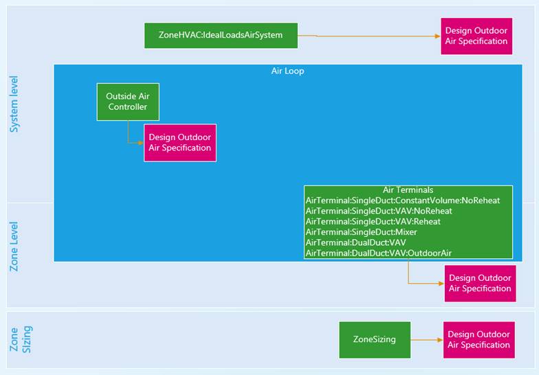
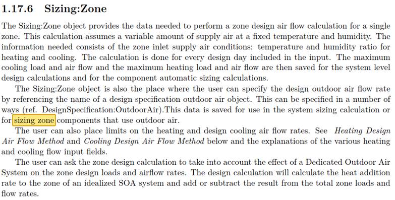
Zone Sizing

The Zone Sizing object allows the definition of data needed for sizing calculations for design days. The description of the object and the relevant parameters are below:

Zone Level

Some air terminals include the option to specify a Design Specification Outdoor Air Object. You can find details on the related property here:

In a similar manner the Ideal loads object can reference these specifications.

System (Air loop) Level

The main component to control outdoor air flow is the Outdoor air Controller.

This controller is a powerful component with quite a range of options, the InputOutputReference.pdf illustrates the following logic:

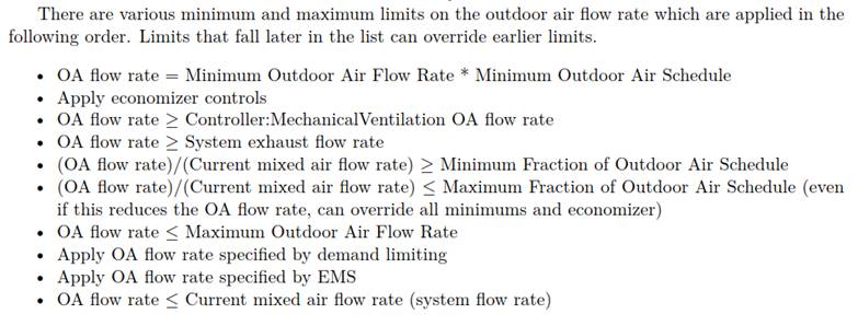
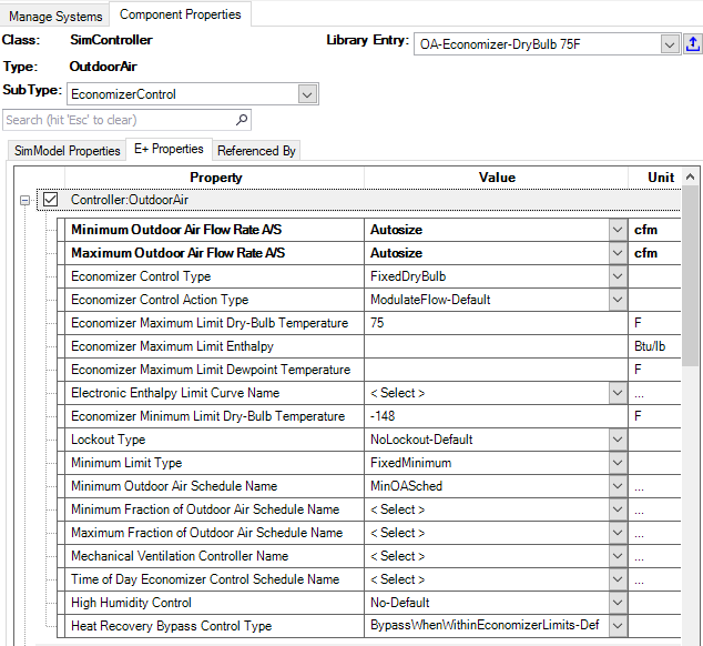
More details on the following parameters:

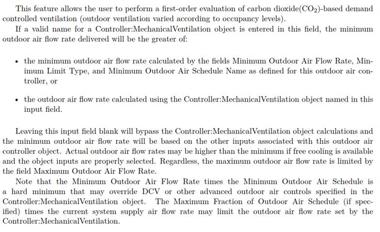
The Mechanical Ventilation Controller specifies one or more design specification objects outdoor air that define outdoor air according to ASHREA 62.1:

Parametric analysis

Simple parametric analysis can be done in Simergy by developing a base model as Design Alternative 1 and developing various design alternations. Those can be done by

1. creating additional design alternatives in the Project workspace
2. using measures in the simulation workspace
3. using parameterized measures in the simulation workspace and choose various values for those parameters in different simulation configurations.
4. any combination thereof

Simergy’s support for OpenStudio measures enables the user to do simple parametric analysis. Each measure can be run and adjust the Simergy model just before the EnergyPlus simulation is performed. These measures are Ruby scripts that use the OpenStudio API to modify the model. These modifications can be small, e.g. just changing one or to parameters of a couple of objects like efficiencies or can make major changes to the model, such as replacing HVAC systems with a totally different HVAC system. These measures can also be parameterized, e.g., to adjust the boiler efficiency by providing the efficiency as a parameter. This way, the same measure can be used to run various scenarios with different measures and measure parameters.

Measure types

Generally, there are three different measure types: Model, EnergyPlus and Report Measures.

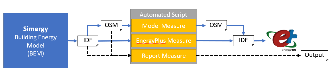
The model measures use the high level OpenStudio API to read and write an OSM file. This simplifies access to the OpenStudio Model but does not cover the full spectrum of all EnergyPlus objects. It also includes an additional conversion process from IDF to OSM and back.

EnergyPlus measures (which we recommend), adjust the model at the EnergyPlus object level (IDF file) and is thus a more direct way of adjusting the model. This direct access to EnergyPlus objects requires version specific code or measures to work with more than one EnergyPlus version.

Report measures are run after the simulation and could be based on either the high level OpenStudio API or the EnergPlus object level API. A report measure collects input and results data and generates a specific report.

Measures in Simergy

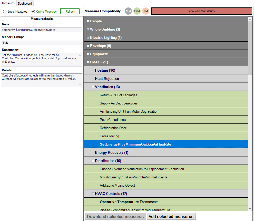
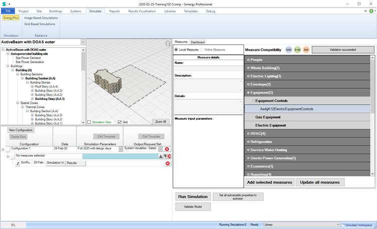
Simergy bundles several measures within the installation. In addition, more measures can be downloaded via the Online Measure functionality in Simergy V4.0.

The Simergy Local Measure UI lists all locally available measures in a predefined taxonomy and the user can with drag and drop measures onto a simulation configuration or use the “Add selected measures” button. Once a measure is attached to a simulation configuration, its parameters can be adjusted.

Each configuration can have its own set of measures and related parameters. Through adjusting the measures and their parameters across various simulation configurations and/or design alternatives, a parametric analysis can be performed.

Online Measures

With Simergy Version 4.0, Simergy supported downloading of measures from BCL (Building Component Library). The measures are organized on the mentioned topology and can be downloaded and used with a button click.

Measure validation

When entering the Simulation Workspace, Simergy performs a validation check if all objects used in the model are also supported by the OpenStudio API. If issues are found, they can be reviewed in the following dialog and only EnergyPlus and some Report Measures area available for selection.

Feedback from Measures

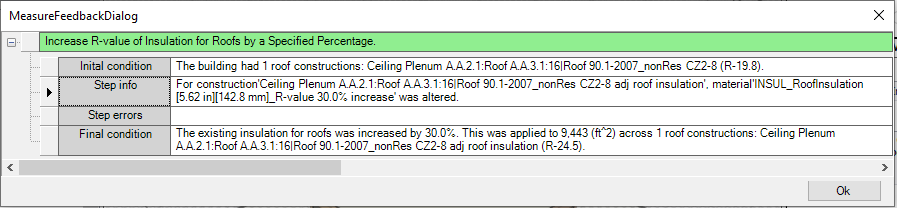
Details about each measure run can be found by clicking on the successful/error button on each measures row.

Reports and Results Visualization

All results generated in either form, with design alternatives, measures, or combinations thereof, can be viewed within Simergy in reports and in results visualization the same way any simulation results can be viewed.

Writing your own Measures

Besides using existing measures, users can also write their own measures. A reference guides is available here:

https://nrel.github.io/OpenStudio-user-documentation/reference/measure_writing_guide/

Once the general measure structure is setup it is as easy as writing ruby code and using the OpenStudio Model API.

https://openstudio-sdk-documentation.s3.amazonaws.com/cpp/OpenStudio-2.9.0-doc/model/html/index.html

Simergy – autosizing of component parameters

Capacity and flow rate parameters can usually be autosized (indicated by the A/S postfix to the parameter name). Note that most of the default templates and library entries have the properties set to autosize.

If you set one or more properties to autosize you also need to provide design days, which are used for the sizing calculations in EnergyPlus. In addition, sizing objects at the Zone Group Occupancy template, air loops and water loops define more specifics about the sizing calculation. Autosizing related objects:

• Design days (typically two summer and one winter design day)
  Note: If you select a standard weather source, those three design days are automatically attached to your project.
• Zone Sizing
• Air Loop Sizing
• Plant Loop Sizing
• Global Sizing

See an example of each below:

                                                               Design days in the location template in the Site workspace

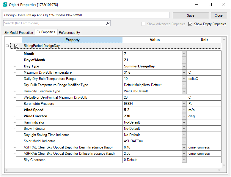
                                                     Design days properties in the Object Properties dialog

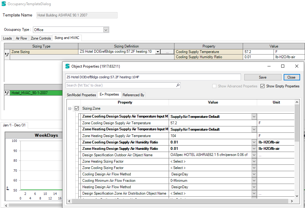
                                                                                    Zone sizing dialog in occupancy template

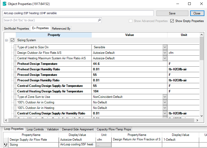
                                                                              Air loop sizing dialog

                                                                          Water loop sizing dialog

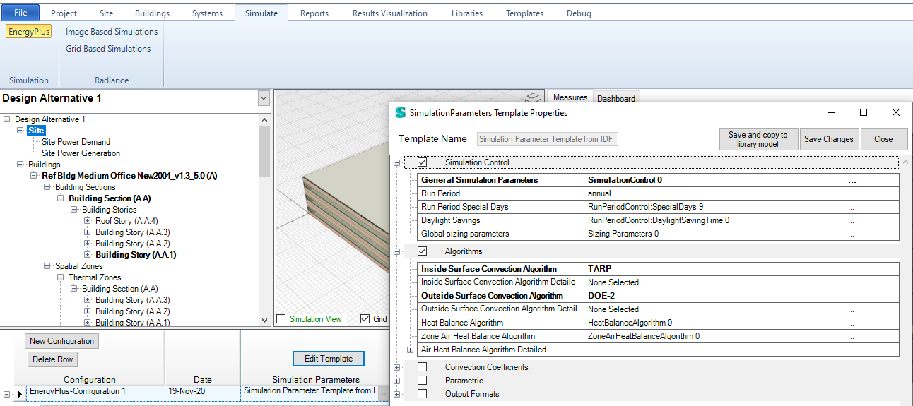
                                                      Global Sizing Parameters in the Simulation Parameter template in the Simulation workspace

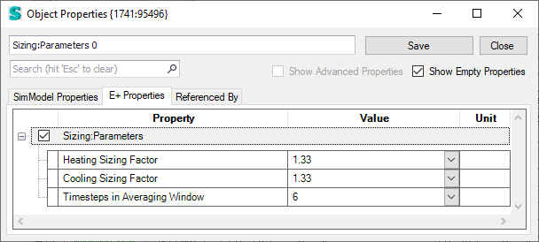
                                     Sizing parameters in the Object Properties dialog

In the simulation workspace you can automatically set all parameters with autosize capabilities to autosize by clicking the   button.

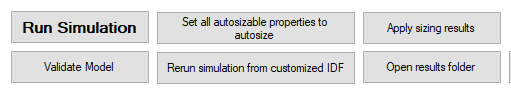
When you click the  button, you can apply the sizing results to your model. A new window will pop up that shows the full list of properties with calculated values. You can specify a overwrite value and by clicking the “Save values to model” those values are written into the properties.

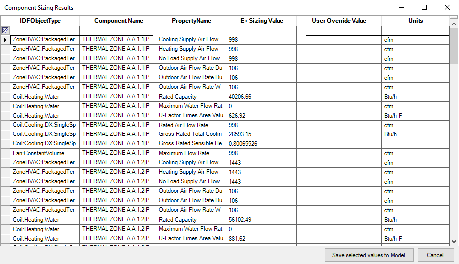
                                                                                                          Sizing results dialog

Under some circumstances, EnergyPlus fails to properly size components and creates error messages that stop the simulation. Is may be possible to adjust the sizing object values to resolve this issue or by setting these autosize properties to specific values so the sizing and simulation can run through. After the simulation completes you can reapply the sizing values to get better estimates.

You can either create your own measures or download the from the building component library: https://bcl.nrel.gov/

Download the zipped file and extract all files into the following directory:

C:\Users\Public\Simergy\LibrariesAndTemplates\Measures

with the parent measure folder.

The measures then show up automatically in the Simulation workspace in the Measures tab.

Note that not all measures do always show up, since we perform a compatibility/validation check if your current model is OpenStudio API capable. If not the ModelMeasures (MM in blue) are hidden.

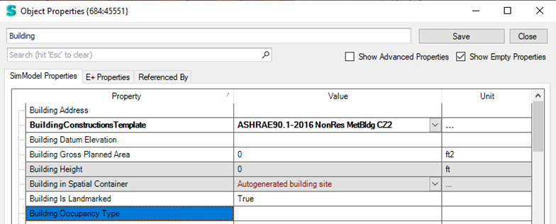
Setting the Building Type

The Building Type is inferred from the Project Type (e.g., "Office Project Type" -> "Office)

• The user can overwrite this Building Type by setting a value to the
  Building Occupancy Type property of the building object. Just select the building in the project tree, right click and select Properties.

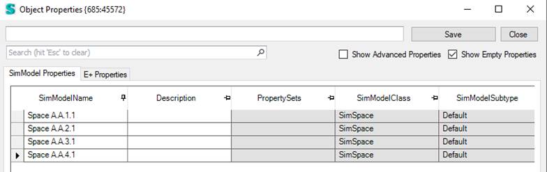
Setting the Space Type

The Space Type is derived from the above Building Type and by default set to a meaningful value.

• The user can overwrite this Space Type by setting a value to the Description property of a space. Select a space in the tree, right click an either select Properties to edit the selected space or select Edit Space in Table to edit all the spaces in your model in a table view (see below).

The Building and Space Type get exported then to the OSM model by assigning them to the space type.

In Simergy V4.1, we will add a more straight forward way to enter/select those types.

Inject IDF snippets

Sometimes it is useful to quickly inject IDF snippets in the IDF file that is generated by Simergy. Adding report variables or meters for example is a use case for this.

When you place an IDF file named “InjectIDF.idf” into the same folder as your simp file, Simergy will automatically add the content of that IDF file into the generated IDF file. Anything can be added that corresponds to correct IDF Syntax. 

Many Simergy users are outside the US, so the Standard weather data provided in Simergy is not useful to them.  Instead they use the “Custom” option for Weather data.  If such users copy their weather data files (EPW/DDY/STAT) to the folder C:\Users\Public\Simergy\WeatherFiles – then Simergy will find them when the “Custom” option is selected – as shown below:

EPW files exist for hundreds of locations around the world, but it is sometimes difficult to locate DDY (Design Day) files for those locations. 

This FAQ describes the process for defining Days and associating them with a location in Simergy.

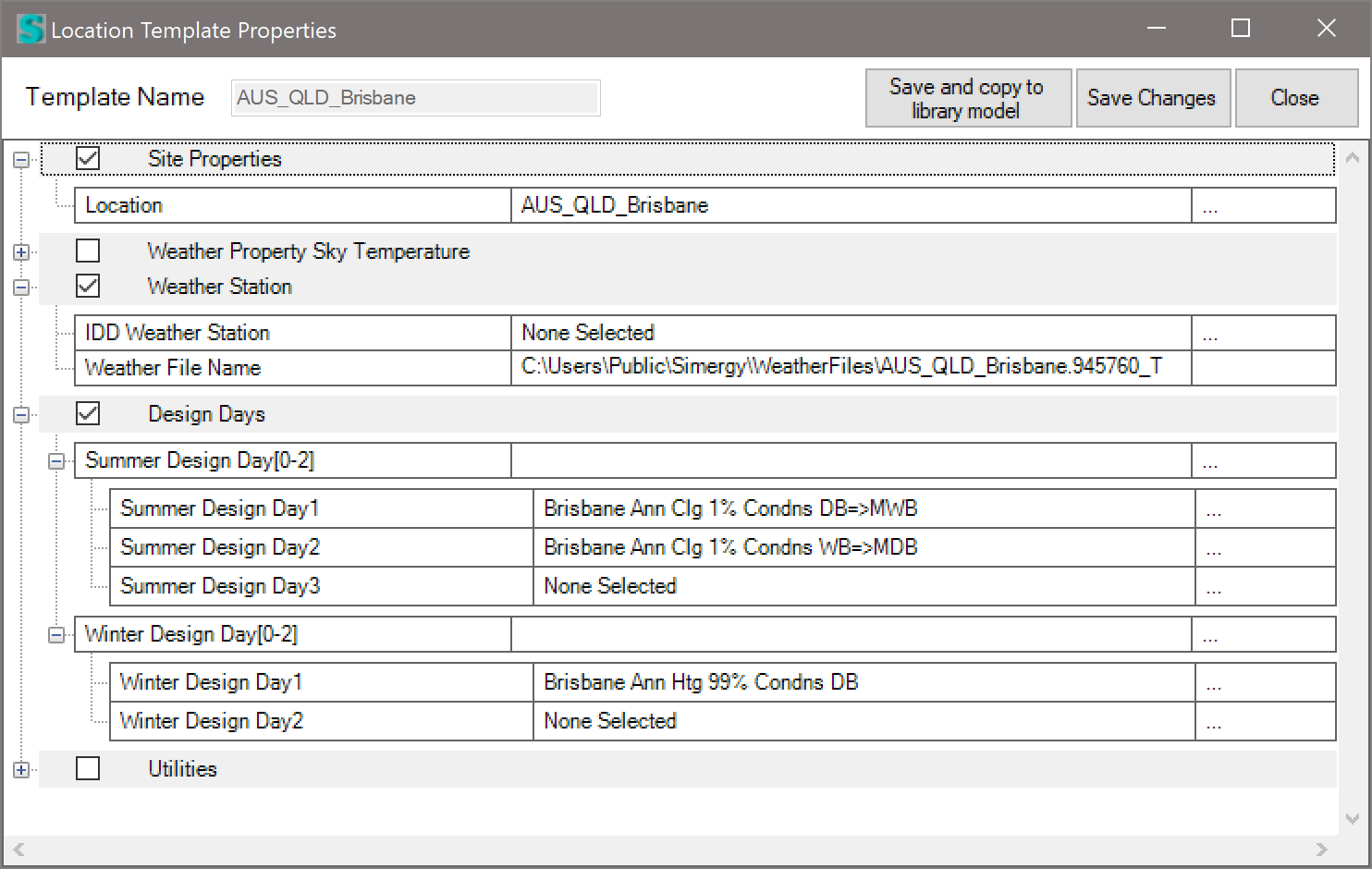
1. After selecting your EPW file, go to the Site workspace > select the building site object in and of the following views – Tree, 3D, 2D plan (as shown below)
   
   
   
2. At the very bottom of the application frame, you will see the Library that is selected (“Library” by default). If you put your Design Days in the default library (“Library.siml”), then you don’t need to change it.  If you put them in a different library, then select it in the dropdown list.
   
   
   
3. Now look to the left, near the bottom for something like “AUS_QLD_Brisbane” – and an “Edit” button > click the Edit button, and you will see the location template that was created when you selected the custom weather file – shown below with the empty Summer and Winter design day lists expanded:
   
   
   
4. Where it says “None Selected” > click the dropdown list and it will show you the available Design Days in both the Project model and in the Library (red text). Select the design day you want first, then select second, and so on.  When you have selected all you want > click “Save Changes” and then “Close.”  The design days are now associated with this location.

NOTE: Having explained the hard way to do this.  I see that you already added your design days into the DDY file associated with your EPW file.  So the easy way to do it is to copy your (3) files into the weather data folder (C:\Users\Public\Simergy\WeatherFiles) and then re-select it with the custom weather ‘Browse’ feature shown above.  If the DDY file has Design Day data in it – all of the above will be done for you automatically

Here is what I got using your data:

What are unmet load hours?

Unmet load hours are hours where, for some reason, the thermal loads in a space cannot be satisfied by either the heating or the cooling system. There can be many reasons for unmet load hours, including: systems being too small, not controlled correctly, not reacting fast enough, loads are especially high or low, or do change dramatically, schedules out of sync, unrealistic U-Values, etc.  Typically, these conditions cannot be eliminated, but can be reduced to an acceptable level.  Therefore, when talking about unmet load hours, we first need to define what threshold of unmet load hours is considered to be acceptable. A commonly used threshold for unmet load hours is to not exceed 300 hours (ASHRAE Standard 90.1).

Digital Alchemy, has developed the following process flow – for reducing unmet load hours:

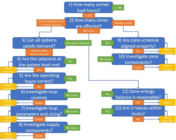
This process flow helps users to start investigating unmet load hours in a structured way. Not all steps have to be completed in this order. This process is rather a guideline to follow. In some cases, it will become clear after addressing a couple of questions what is the root cause and thus needs to be adjusted. The sections below provide more detail about each of these questions.

1)     How many unmet load hours?

The Project Summary Report contains two indicators for heating and cooling unmet load hours.

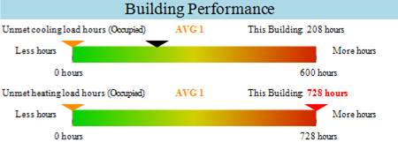
In this example we clearly have an issue with unmet heating load hours, whereas the unmet cooling load hours are acceptable.

2)     How many zones are affected?

It can be very useful to determine which zones are affected and are creating the most unmet load hours. There are two reports that you can use to find an answer to this question: Temperature Profile Report and Setpoint Not Met Report.

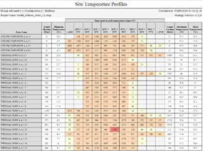
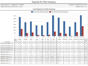
You should see in both if you have unmet load hours in random zones or just for specific floors or grouped by systems. If they are affecting most of the zones or they are related to one or more systems, we should look at the system level next, if only a few zones are causing the high unmet load hours, then we can focus just on these zones of the building and skip to question 9.

3)     Can all systems satisfy demand?

Based on the understanding which areas of the building have the most unmet load hours, it is usually easy to identify the related systems. The best way to understand if a system can satisfy demand is to investigate additional variables in the Results Visualization workspace. For example, to look at the systems Unmet Demand Rate or the Not Distributed Demand Rate in context of the Heating/Cooling Demand Rate. Those are included in most output request sets and can be easily drawn in the results visualization workspace.

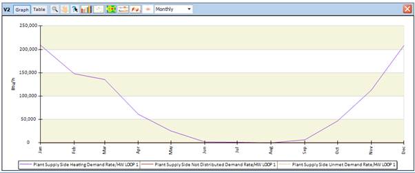
In this example, the unmet and not distributed numbers are very low and appear to be 0 compared to the actual demand rate.

4)     Are the setpoints at the system level met?

In the Model Assessment Report, you can find a graph on Setpoint Achievement and quickly determine if there are any loops where the setpoint and the actual temperature differ drastically. Note that this is a stagged area graph, so values are added and show the temperature difference.

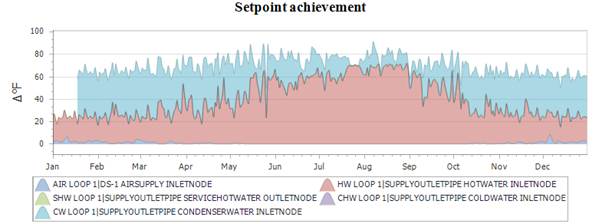
In this graph, we see high temperature differences for the hot water loop especially in the summer and high temperature differences for the CW Loop in the winter.

Another way to look temperature setpoints is to graph the supply temperature and the related setpoint in the Results Visualization workspace.

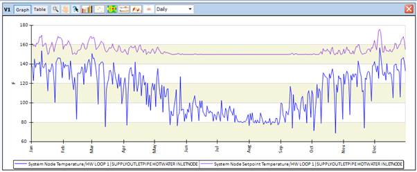
This is the same HW Loop then in the Model Assessment Report above and shows again the large discrepancy in the summer. These kinds of differences indicate that the setpoint cannot be met. This would explain the unmet demand we detected earlier. To determine what is causing this, we need to investigate the next 4 questions to determine the exact reason for this difference (incorrect operating hours, incorrect loop controls, insufficient loop parameters or sizing or incorrect component parameters).

5)     Are the operating hours correct?

In the Model Assessment Report, you can find a graph of operating hours that can help to identify if certain systems are not operating at times when they should be operating.

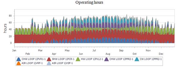
In this example, we can see a weekday - weekend pattern for most loops. In addition, we can see the typical summer/winter patters for hot and chilled water loops.

6)     Investigate loop controls

One potential reason for setpoint differences is the loop level controls. Assuming that the supply temperature controller is specifying the correct temperature, we need to look at the availability managers and the plant operation schemes. If availability managers do turn of systems, we should have seen the effect in the previous operating hours graph. Whereas the plant operating schemes define which supply components are operating under specific load conditions. For simple loops this is straight forward, whereas for more complex loops especially mixed water loops you need to ensure a correct definition.

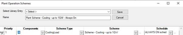
This image shows the plant operation scheme for a chilled water loop using all chillers up to a cooling load of 1GW.

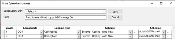
This image shows a plant operation scheme for a mixed water loop that assigns a cooling scheme for a district cooling component and a heating scheme for a district heating component both at 1 GW.

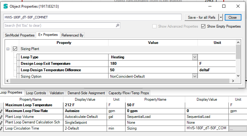
7)     Investigate loop parameters and sizing

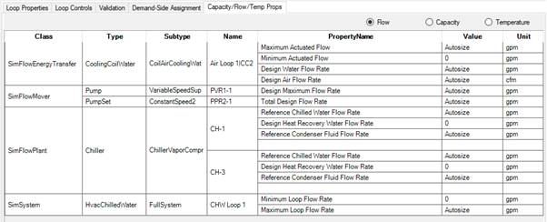
Another potential source of error could be the loop parameters and its sizing. Loop parameters are for example specifying a Maximum Flow Rate. Typically, this is autosized, but if it is hardsized this may be the source of the unmet load hours. Gradually increasing the hardsized flow rates will show if this is the limiting factor. When looking at the loop flow rate, it is also beneficial to investigate the flow rates of all components in the loop and see if there are any discrepancies. There is a special tab that summaries flowrates, capacities, and temperatures of all components in a loop:

In this example the flow rates are all autosized, so we would investigate the sizing parameters next. The sizing properties for water loops typically define an exit temperature and a temperature difference. You should make sure the exit temperature matches your supply setpoint controllers’ temperature. If that is appropriate, you can adjust the temperature difference to finetune the sizing results. Whereby a smaller temperature difference would lead to increased component sizes.

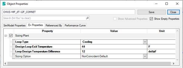
This example shows typical sizing parameters for a chilled water loop.

8)     Investigate supply components

If none of the above questions helped with decreasing the unmet load hours, you should look at the supply components in that loop next. Are those properties aligned with the loop level properties? Are flow rates and temperatures consistent. Does the component have any local controls that may cause it to work at lower capacity or not at all? What exactly the cause of a misbehaving component is depends on its type, but it is usually a good idea to start with its operating status, flow rate and inlet and outlet temperatures.

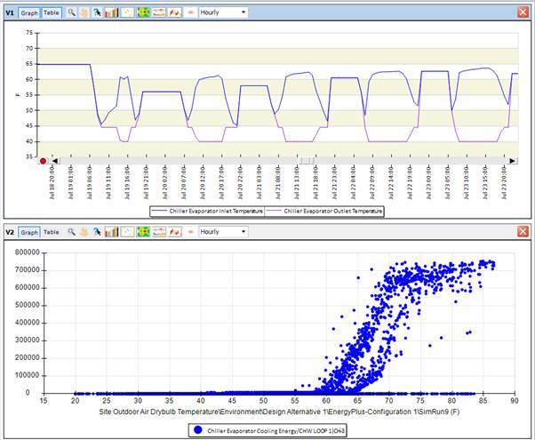
These two examples show chiller evaporator inlet and outlet temperature in the upper graph zoomed in and evaporator cooling energy in a scatter plot over outside air temperature. The later nicely shows that with increasing outside air temperature the cooling energy increases until it seems to hit a maximum capacity around 70 deg F OAT. Maybe the chiller size is too small?

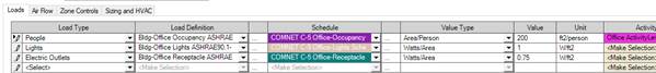
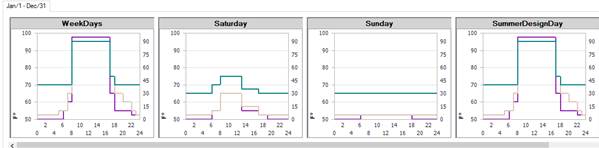
9)     Are zone schedules aligned properly?

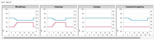
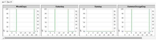
In the Building workspace, click on Zone Load Groups and then on edit template Values. The schedules for this collection of templates are shown graphically (below).  This enables you to see if the schedules are properly aligned. Specifically, the internal loads versus the Zone Controls and the HVAC availability schedule. For example, if an HVAC availability schedule is starting too late in the day (an hour later than the internal loads schedule) then we can expect to see unmet load hours at those times of the morning.

10)  Investigate zone components

Similarly, to the system components, the zone components can also limit the energy flow and thus cause unmet load hours. In this area it is also difficult to give direct advice other than to investigate variables of those components and look for decreased performance indicators, low flow rates, low energy consumption, etc. Ones a component is identified as being undersized, you should gradually increase its size and verify that the unmet load hours are decreasing.

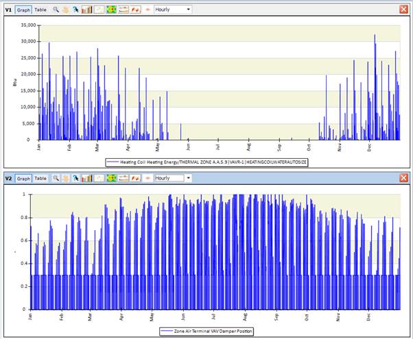
These two graphs show details of an air terminal, the lower graph show the VAV Damper position. It seems fine fluctuating between 0 and the minimum of 0.3 and depending on the demand up to 1.0 setting at some days in the summer. The heating energy graph of the related coil also looks reasonable, showing heating energy in the winter.

11)  Is the energy balance reasonable?

In the Model Overview report, the zone energy balance shows the gains and losses forming an energy balance. This is useful to understand the buildings behavior. Generally, the different categories should be compared to identify either categories with a very low or a very high influence on the energy balance. Obviously, this balance is a very characteristic graph for each individual building.

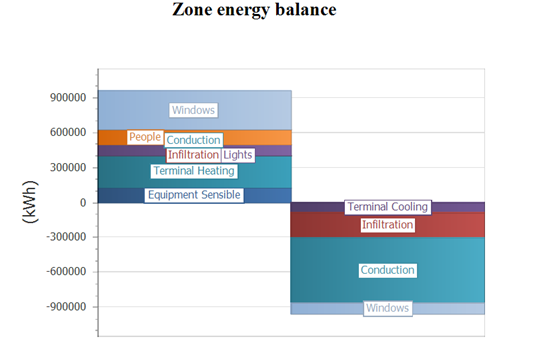
This example shows that the Conduction and Infiltration are very low on the heat gain side (left), whereas they are the two largest portions on the heat loss side (right). Similarly, the terminal cooling is relatively small compared to the terminal heating and equipment sensible. This leads to the assumption that this building is heating dominated. In other words, this graph puts different aspects of gains and losses into perspective and could hint to areas that need further investigation.

12) Are the material/construction U-Values reasonable?

In the Model Overview report, the U-Value overview report shows minimum, average, and maximum U-Value for each building element. This allows for a quick verification that the U-Value lies in the expected range and that no outliers are defined anywhere. If you see any problems in the report the Envelope Summary report provides a lot more details on the envelope.

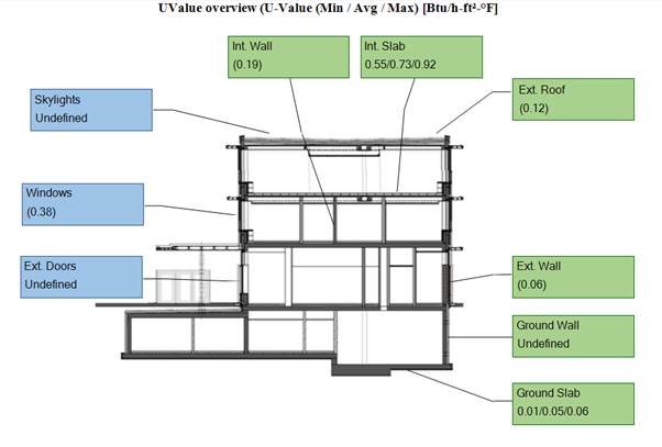
This U-Value overview report does not contain any outliers since all U-Values are smaller than 1 Btu/h-ft²-F.

References:

We developed this document based on our experience with EnergyPlus and Simergy. You may find more hints if all the above did not provide and insight on where you need to improve your model.

Report with monthly electricity results

Open the Project Comparison Report, on page 2 you can find “Total Monthly Electrical Consumption (kWh)” and on page 3 you can find “Total Monthly Electrical Demand (W)”. This is a report that shows one or more design alternatives and simulation runs so you can compare those against each other. See screenshot below for an example of the two bar charts and data tables.

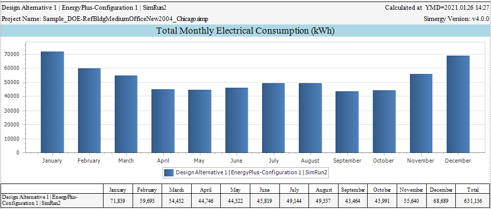
                                                              Project Comparison Report - Total Monthly Electrical Consumption (kWh)

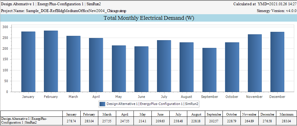
                                                                  Project Comparison Report - Total Monthly Electrical Demand (kW)

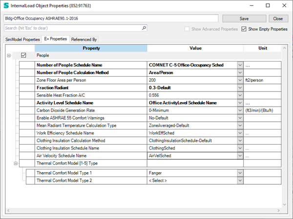
In the libraries workspace

You can find comfort models related output variables like PMV and PPT assigned to the People Type in the Interna loads object:

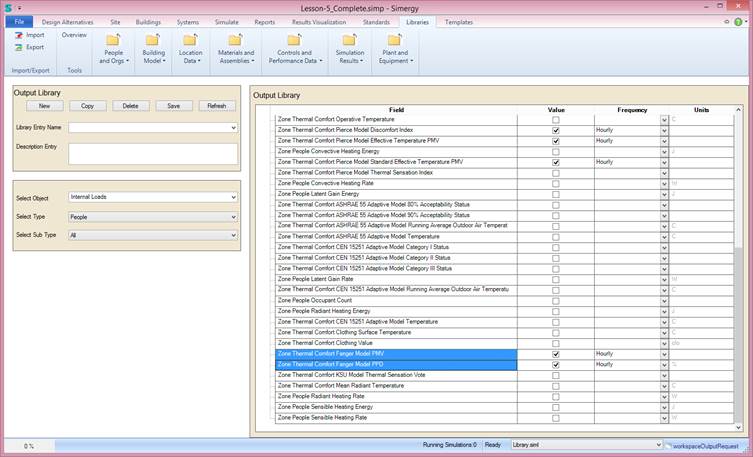
In the Buildings workspace

Be sure that you have properly defined one or more thermal comfort models on the People objects. Go To the Buildings workspace -> Zone Grouping -> Edit Template -> ... button right next to the Occupants. YOu need to select at least one Thermal Comfort Model and the related properties such as Work Efficency, Closing and Air Velocity Schedules.

For more details on those models and the people object properties see: https://bigladdersoftware.com/epx/docs/9-2/input-output-reference/group-internal-gains-people-lights-other.html#people

 Results Visualization with monthly data

In EnergyPlus and Simergy there exists a large range of output variables and output meters. All of which can be either defined in the output requests set template or added to the InjectIDF.idf file.

Typical electricity or gas meters at the facility and building level are as follows:

To better understand which meter sums up other meters, you can refer to the “eplusout.mtd” file that contains all relevant meters for each specific run.

More specific electricity meters are:

Some example for gas meters are:

In order to output electric demand the following variables can be added:

Similar to before the first variable is the sum of the other two (building and HVAC).

 In Simergy Version 4.0, a new output request set template is available that contains all mentioned meters and variables (Electric/gas consumption and demand).

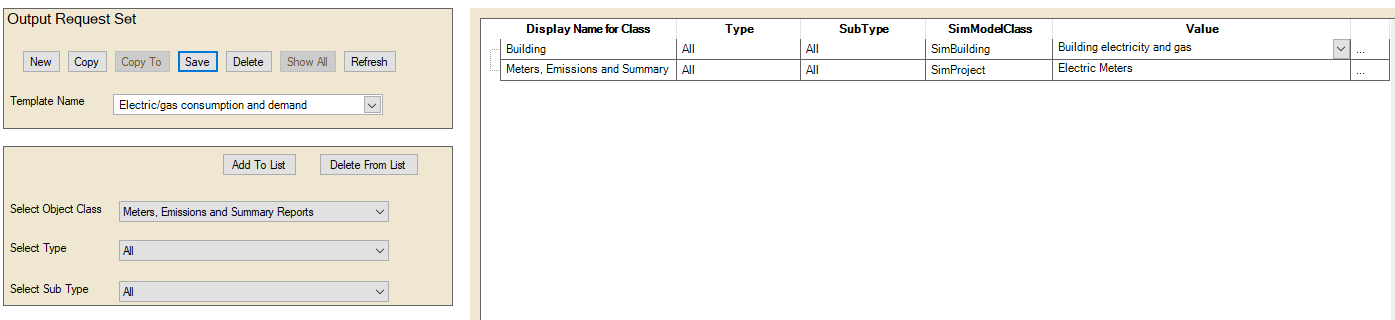
                                                                                                    Templates workspace – Sample output request set template

This template contains one or more output request sets which are also editable, so the user can add or remove meters and output variables. We recommend leaving the Frequency of reporting at its default “hourly” value. The interval is very easily adjusted in the Results Visualization workspace.

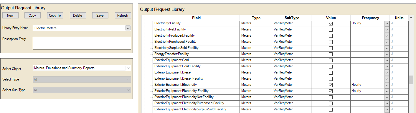
                                                                                                 Library workspace – Sample output request set

Once you assign the output request set to a simulation configuration in the simulation workspace, the variables and meters get added to the IDF file on export. After a successful simulation run they are accessible via the Result Visualization workspace. Below are two bar chart examples showing total electrical demand and total electricity on a monthly interval as well as electrical and gas consumption.

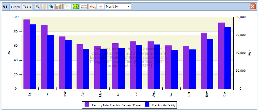
                                                                 Results Visualization – Electrical demand and consumption

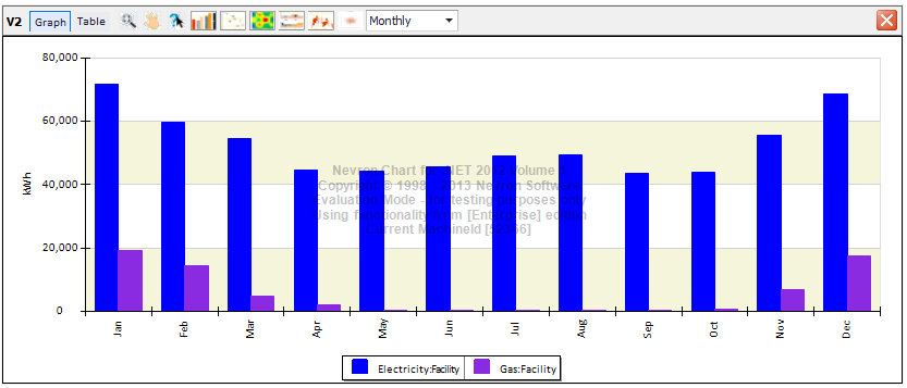
                                                                Results Visualization – Electrical and gas consumption

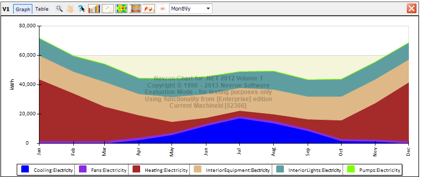
                                             Results Visualization – Stacked area chart of various electricity consumers

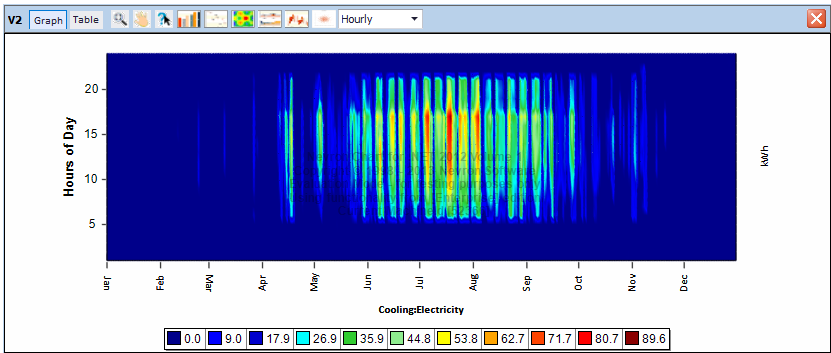
                                          Results Visualization – Scatter chart of electric consumption for cooling

How to create a Green Roof in Simergy

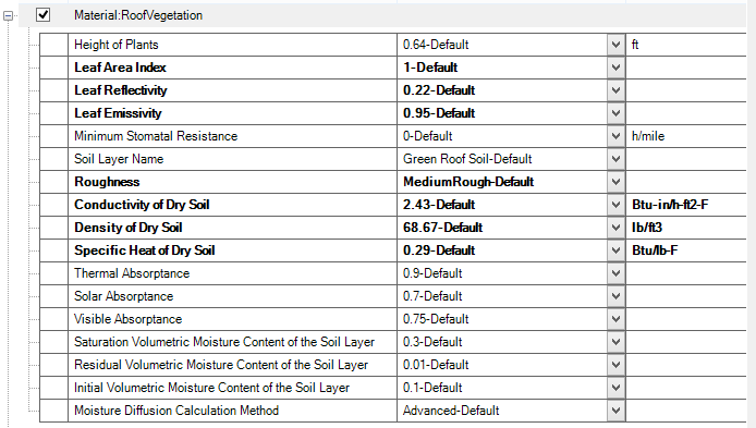
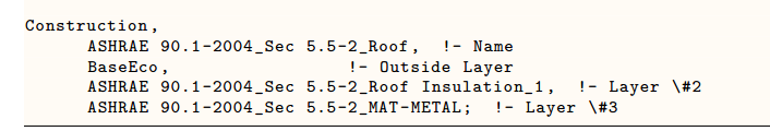
A green roof can be simply created in Simergy by using a special material called Material:RoofVegetation (SimMaterial/OpaqueMaterial/RoofVegatation) as the outside layer of the roof construction (material layer set). Typically, a green roof has a number of additional layers compared to a normal roof for drainage. Depending on your LOD of the model these can be added to the construction.

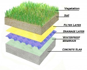
 The following figure shows all properties of the roof vegetation layer

An example of a simplified green roof material layer set:

EnergyPlus documentation suggests that green roofs may require "more timesteps" than normal simulations.

There is a process for transferring content between libraries.  Here is a quick tutorial on that:

1. When installing a new version of Simergy, the ‘Library.siml’ and ‘T24 Library.siml’ files are backed-up to a safe location and new version (companitible with the new Simergy version) are installed. The save location is at: C:\Users\Public.  There you will find folders beginning with “SimergyUserBackup.”  Inside that folder, you will find folders for ‘LibariesAndTemplates’ and ‘ProgramData’ -- as you see below:

    
   
   

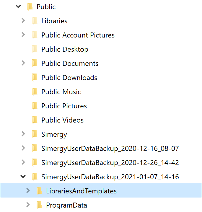
2. To retrieve library entries and templates you created in the previous version > go to the ‘LibariesAndTemplates’ folder and rename ‘Library.siml’ to ‘OLD-Library.siml’ > then copy this library to C:\Users\Public\Simergy\LibrariesAndTemplates folder – with the new ‘Library.siml.’ You could copy you old library content into the new ‘Library.siml’, but the better idea is to create you own library with your content.  To do this > copy the new “TemplateEmptyLibrary.siml” to a new file with a name you give it – e.g. ‘MyLibrary.siml.’  Your ‘LibrariesAndTemplates’ folder should look something like this:

   
   
   

To copy your library entries to ‘MyLibrary.siml’ – do the following:

3. Start Simergy > click on ‘File’, then ‘New’, then ‘Options’, then ‘Library/Template Defaults’ – you should see this:
   
   
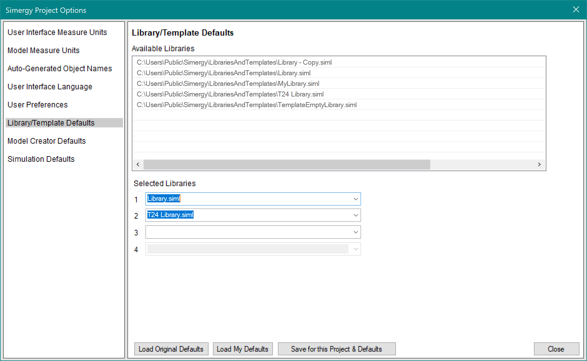
4. Now click in the Selected Libraries 3 dropdown list and select OLD-Library.siml and/or ‘MyLibrary.siml’ – and if you want both to become available – add the other one in library slot 4. If you did both of those things, you will see this:
   
   
   

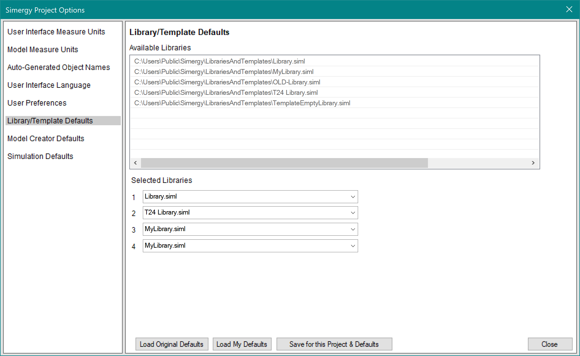
   Click on ‘Save for this Project & Defaults’

   Now all 4 of these libraries will be available to you whenever you are using Simergy.

5. Now go to Libraries > select the library (lower right) that has the content you want to copy >
   • To copy individual library entries > select them in the ‘Library Entry Name’ field and then click on the ‘Copy To’ button above the library entry name – like this:
     
     
      
     This will surface a dialog in which you select the library to which you want to copy this entry – like this:
     
     
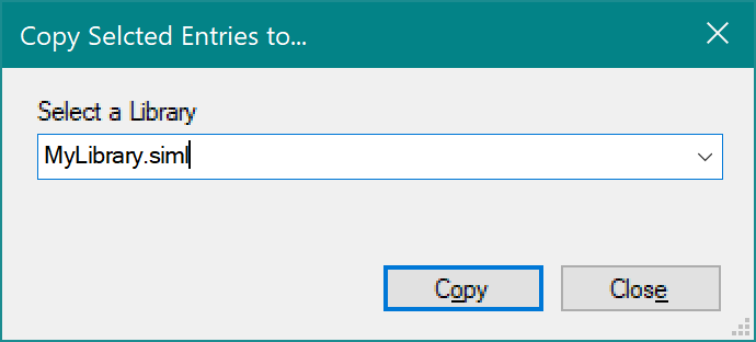
   • To copy many library entries at one time > Click on the ‘Show All’ button above the ‘Library Entry Name.’ A table with all the library entries will be generated and shown:
     
     
     

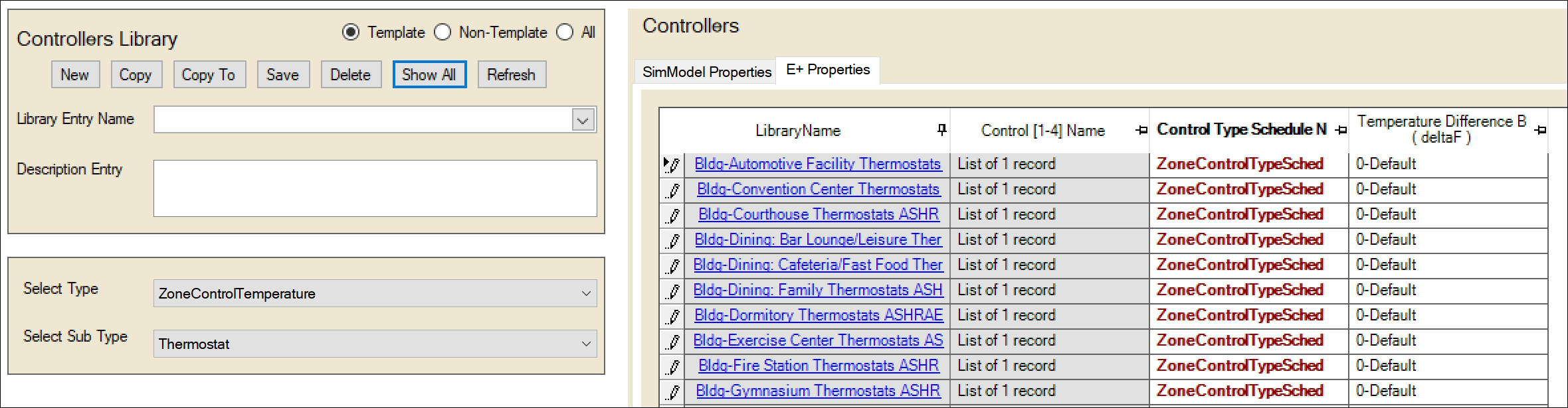
     Select the entries you want to copy > then click on ‘Copy To’ – which will give you the same dialog as how above to select the library to which you want to copy these entries.

      

      

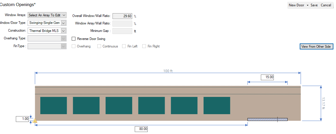
Establishing thermal bridge parameters

With a tool like LBNL’s Therm, you can determine basic parameters about thermal bridges, such as area, thickness, and thermal resistance.

https://windows.lbl.gov/tools/therm/software-download

 Defining the thermal bridge material layer set

• Go to the Library workspace
• Select MLS Editor
• Press the New button
• Select OpaqueLayerSet as Type
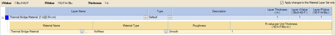
• Select NoMass as MaterialType for the first layer in the MLS grid on the right and specify a material name, thickness, R-Value per Thickness and Roughness value and Save. 
  
  

Apply thermal bridge material layer set

• Go to Building workspace
• Select Custom Openings
• Select a wall in the 3D view (or the 2D view or the tree)
• Click on New Door and place the “door” representing your thermal bridge in context of the wall.
• Change the Construction to the Thermal Bridge MLS you created above.