How can I reduce unmet load hours?
What are unmet load hours?
Unmet load hours are hours where, for some reason, the thermal loads in a space cannot be satisfied by either the heating or the cooling system. There can be many reasons for unmet load hours, including: systems being too small, not controlled correctly, not reacting fast enough, loads are especially high or low, or do change dramatically, schedules out of sync, unrealistic U-Values, etc. Typically, these conditions cannot be eliminated, but can be reduced to an acceptable level. Therefore, when talking about unmet load hours, we first need to define what threshold of unmet load hours is considered to be acceptable. A commonly used threshold for unmet load hours is to not exceed 300 hours (ASHRAE Standard 90.1).
Digital Alchemy, has developed the following process flow – for reducing unmet load hours:
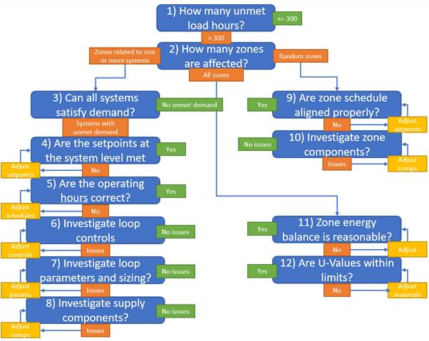
This process flow helps users to start investigating unmet load hours in a structured way. Not all steps have to be completed in this order. This process is rather a guideline to follow. In some cases, it will become clear after addressing a couple of questions what is the root cause and thus needs to be adjusted. The sections below provide more detail about each of these questions.
1) How many unmet load hours?
The Project Summary Report contains two indicators for heating and cooling unmet load hours.
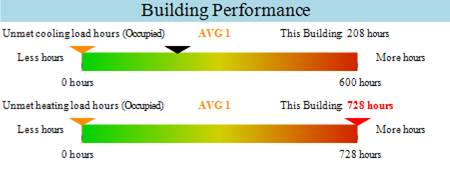
In this example we clearly have an issue with unmet heating load hours, whereas the unmet cooling load hours are acceptable.
2) How many zones are affected?
It can be very useful to determine which zones are affected and are creating the most unmet load hours. There are two reports that you can use to find an answer to this question: Temperature Profile Report and Setpoint Not Met Report.
|
Temperature Profile Report |
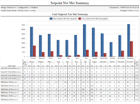
Setpoint Not Met Report |
|
|
|
|
In this report you can find out which zones are most affected and if the problem is on the heating, cooling or both sides. |
Here you can see how the setpoints are not met over the year, what kind (heating and/or cooling) and which zones may be most affected. |
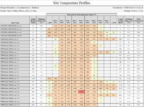
You should see in both if you have unmet load hours in random zones or just for specific floors or grouped by systems. If they are affecting most of the zones or they are related to one or more systems, we should look at the system level next, if only a few zones are causing the high unmet load hours, then we can focus just on these zones of the building and skip to question 9.
3) Can all systems satisfy demand?
Based on the understanding which areas of the building have the most unmet load hours, it is usually easy to identify the related systems. The best way to understand if a system can satisfy demand is to investigate additional variables in the Results Visualization workspace. For example, to look at the systems Unmet Demand Rate or the Not Distributed Demand Rate in context of the Heating/Cooling Demand Rate. Those are included in most output request sets and can be easily drawn in the results visualization workspace.
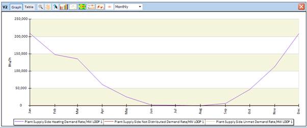
In this example, the unmet and not distributed numbers are very low and appear to be 0 compared to the actual demand rate.
4) Are the setpoints at the system level met?
In the Model Assessment Report, you can find a graph on Setpoint Achievement and quickly determine if there are any loops where the setpoint and the actual temperature differ drastically. Note that this is a stagged area graph, so values are added and show the temperature difference.
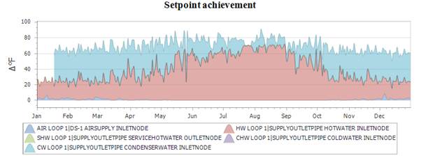
In this graph, we see high temperature differences for the hot water loop especially in the summer and high temperature differences for the CW Loop in the winter.
Another way to look temperature setpoints is to graph the supply temperature and the related setpoint in the Results Visualization workspace.
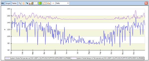
This is the same HW Loop then in the Model Assessment Report above and shows again the large discrepancy in the summer. These kinds of differences indicate that the setpoint cannot be met. This would explain the unmet demand we detected earlier. To determine what is causing this, we need to investigate the next 4 questions to determine the exact reason for this difference (incorrect operating hours, incorrect loop controls, insufficient loop parameters or sizing or incorrect component parameters).
5) Are the operating hours correct?
In the Model Assessment Report, you can find a graph of operating hours that can help to identify if certain systems are not operating at times when they should be operating.
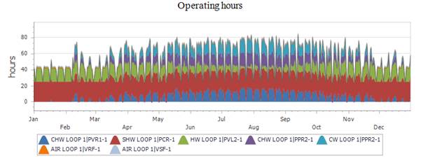
In this example, we can see a weekday - weekend pattern for most loops. In addition, we can see the typical summer/winter patters for hot and chilled water loops.
6) Investigate loop controls
One potential reason for setpoint differences is the loop level controls. Assuming that the supply temperature controller is specifying the correct temperature, we need to look at the availability managers and the plant operation schemes. If availability managers do turn of systems, we should have seen the effect in the previous operating hours graph. Whereas the plant operating schemes define which supply components are operating under specific load conditions. For simple loops this is straight forward, whereas for more complex loops especially mixed water loops you need to ensure a correct definition.
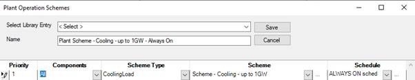
This image shows the plant operation scheme for a chilled water loop using all chillers up to a cooling load of 1GW.
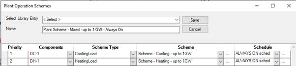
This image shows a plant operation scheme for a mixed water loop that assigns a cooling scheme for a district cooling component and a heating scheme for a district heating component both at 1 GW.
7) Investigate loop parameters and sizing
Another potential source of error could be the loop parameters and its sizing. Loop parameters are for example specifying a Maximum Flow Rate. Typically, this is autosized, but if it is hardsized this may be the source of the unmet load hours. Gradually increasing the hardsized flow rates will show if this is the limiting factor. When looking at the loop flow rate, it is also beneficial to investigate the flow rates of all components in the loop and see if there are any discrepancies. There is a special tab that summaries flowrates, capacities, and temperatures of all components in a loop:
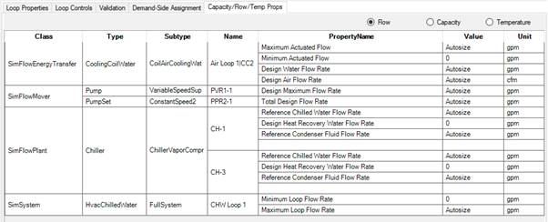
In this example the flow rates are all autosized, so we would investigate the sizing parameters next. The sizing properties for water loops typically define an exit temperature and a temperature difference. You should make sure the exit temperature matches your supply setpoint controllers’ temperature. If that is appropriate, you can adjust the temperature difference to finetune the sizing results. Whereby a smaller temperature difference would lead to increased component sizes.
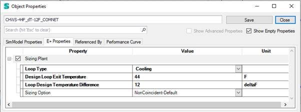
This example shows typical sizing parameters for a chilled water loop.
8) Investigate supply components
If none of the above questions helped with decreasing the unmet load hours, you should look at the supply components in that loop next. Are those properties aligned with the loop level properties? Are flow rates and temperatures consistent. Does the component have any local controls that may cause it to work at lower capacity or not at all? What exactly the cause of a misbehaving component is depends on its type, but it is usually a good idea to start with its operating status, flow rate and inlet and outlet temperatures.
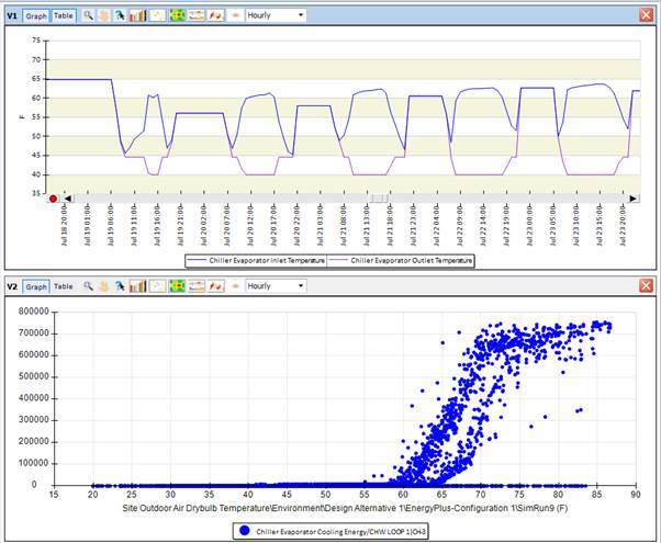
These two examples show chiller evaporator inlet and outlet temperature in the upper graph zoomed in and evaporator cooling energy in a scatter plot over outside air temperature. The later nicely shows that with increasing outside air temperature the cooling energy increases until it seems to hit a maximum capacity around 70 deg F OAT. Maybe the chiller size is too small?
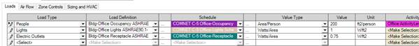
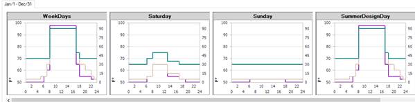
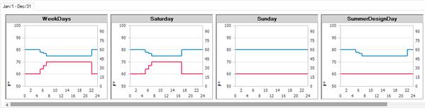
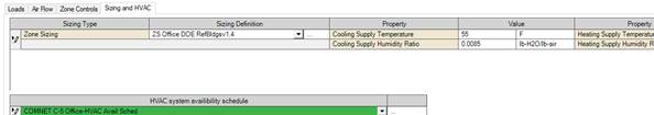
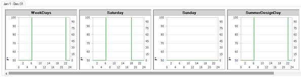
9) Are zone schedules aligned properly?
In the Building workspace, click on Zone Load Groups and then on edit template Values. The schedules for this collection of templates are shown graphically (below). This enables you to see if the schedules are properly aligned. Specifically, the internal loads versus the Zone Controls and the HVAC availability schedule. For example, if an HVAC availability schedule is starting too late in the day (an hour later than the internal loads schedule) then we can expect to see unmet load hours at those times of the morning.

10) Investigate zone components
Similarly, to the system components, the zone components can also limit the energy flow and thus cause unmet load hours. In this area it is also difficult to give direct advice other than to investigate variables of those components and look for decreased performance indicators, low flow rates, low energy consumption, etc. Ones a component is identified as being undersized, you should gradually increase its size and verify that the unmet load hours are decreasing.
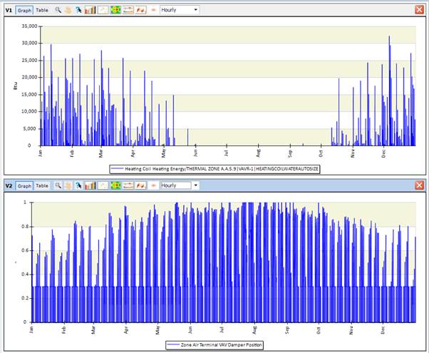
These two graphs show details of an air terminal, the lower graph show the VAV Damper position. It seems fine fluctuating between 0 and the minimum of 0.3 and depending on the demand up to 1.0 setting at some days in the summer. The heating energy graph of the related coil also looks reasonable, showing heating energy in the winter.
11) Is the energy balance reasonable?
In the Model Overview report, the zone energy balance shows the gains and losses forming an energy balance. This is useful to understand the buildings behavior. Generally, the different categories should be compared to identify either categories with a very low or a very high influence on the energy balance. Obviously, this balance is a very characteristic graph for each individual building.
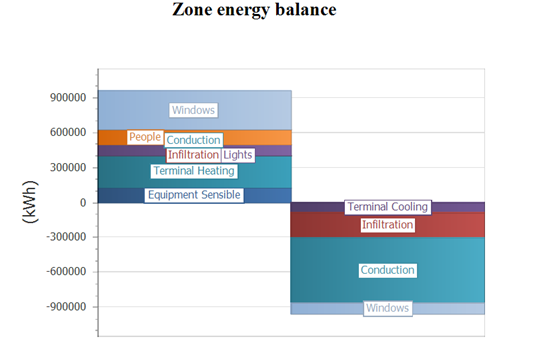
This example shows that the Conduction and Infiltration are very low on the heat gain side (left), whereas they are the two largest portions on the heat loss side (right). Similarly, the terminal cooling is relatively small compared to the terminal heating and equipment sensible. This leads to the assumption that this building is heating dominated. In other words, this graph puts different aspects of gains and losses into perspective and could hint to areas that need further investigation.
12) Are the material/construction U-Values reasonable?
In the Model Overview report, the U-Value overview report shows minimum, average, and maximum U-Value for each building element. This allows for a quick verification that the U-Value lies in the expected range and that no outliers are defined anywhere. If you see any problems in the report the Envelope Summary report provides a lot more details on the envelope.
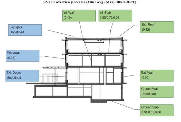
This U-Value overview report does not contain any outliers since all U-Values are smaller than 1 Btu/h-ft2-F.
References:
We developed this document based on our experience with EnergyPlus and Simergy. You may find more hints if all the above did not provide and insight on where you need to improve your model.
|
COMNET advice on unmet load hours |
|
|
6 tips for Reducing Unmet load hours |
http://energy-models.com/blog/6-tips-reducing-unmet-load-hours |
|
Related topics on unmethours.com |
https://unmethours.com/question/359/what-are-your-techniques-for-reducing-unmet-hours/ https://unmethours.com/question/525/tolerance-for-unmet-load-hours-for-leed/ |